Video
Watch the full video
Annotated Presentation
Below is an annotated version of the presentation, with timestamped links to the relevant parts of the video for each slide.
Here is the slide-by-slide annotated presentation based on the video “From Vectors to Agents: Managing RAG in an Agentic World” by Rajiv Shah. This was presented in different forms at several conferences in the Fall of 2025 including, MLOps World | GenAI Summit 2025 and Fully Connected London from Weights and Biases.
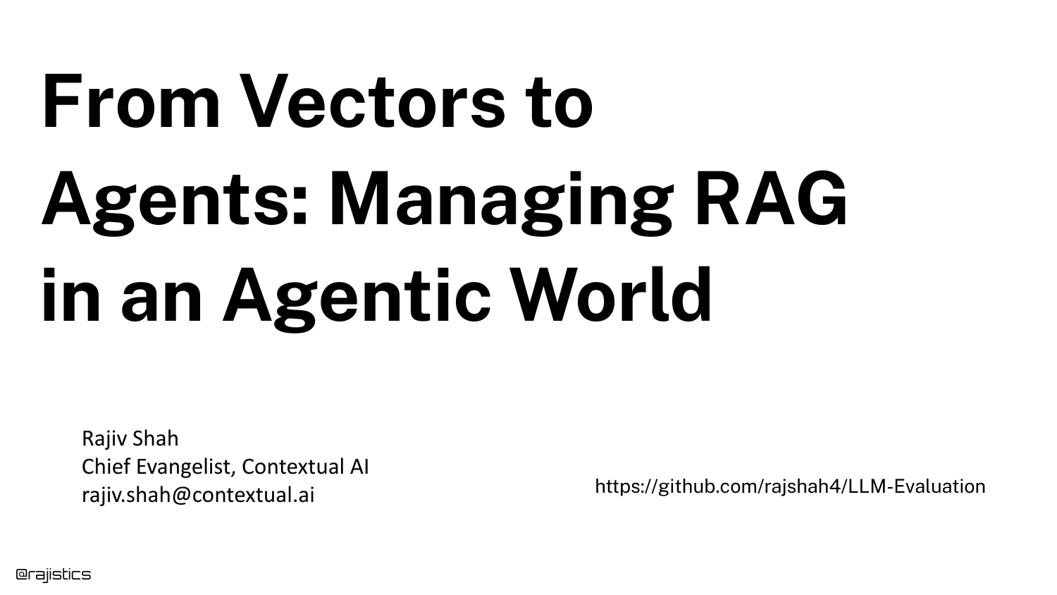
1. Title Slide

The presentation begins with the title slide, introducing the core theme: “From Vectors to Agents: Managing RAG in an Agentic World.” The speaker, Rajiv Shah from Contextual, sets the stage for a technical deep dive into Retrieval-Augmented Generation (RAG).
He outlines the agenda, promising to move beyond basic RAG concepts to focus specifically on retrieval approaches. The talk is designed to cover the spectrum from traditional methods like BM25 and Language Models to the emerging field of Agentic Search.
2. ACME GPT
This slide displays a stylized logo for “ACME GPT,” representing the typical enterprise aspiration. Companies see tools like ChatGPT and immediately want to apply that capability to their internal data, asking questions like, “Can I get the list of board of directors?”
However, the speaker notes a common hurdle: generic models don’t know enterprise-specific knowledge. This sets up the necessity for RAG—injecting private data into the model—rather than relying solely on the model’s pre-trained knowledge.
3. Building RAG is Easy
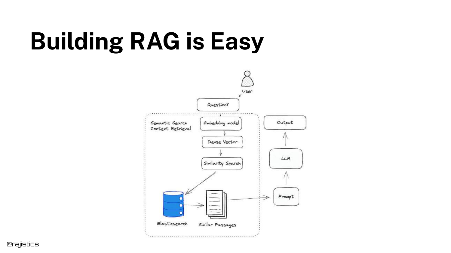
The speaker illustrates the deceptively simple workflow of a basic RAG demo. The diagram shows the standard path: a user query is converted to vectors, matched against a database, and sent to an LLM.
Shah acknowledges that building a “hello world” version of this is trivial. He notes, “You can build a very easy RAG demo out of the box by just grabbing some data, using an embedding model, creating vectors, doing the similarity.”
4. Building RAG is Easy (Code Example)
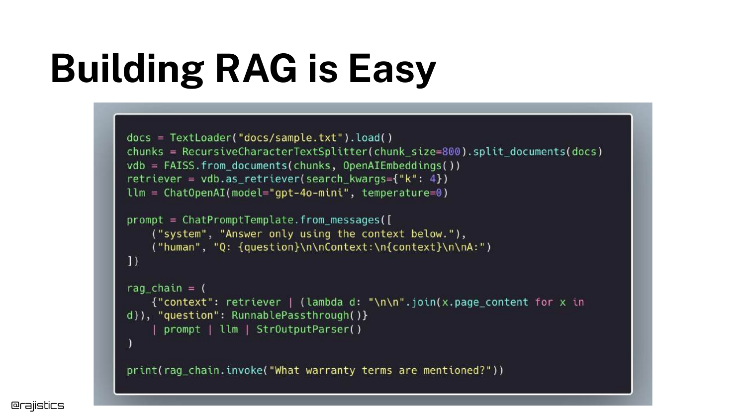
A Python code snippet using LangChain is displayed to reinforce how accessible basic RAG has become. The code demonstrates loading a document, chunking it, and setting up a retrieval chain in just a few lines.
This slide serves as a foil for the upcoming reality check. While the code works for a demo, it hides the immense complexity required to make such a system robust, accurate, and scalable in a real-world production environment.
5. RAG Reality Check

The tone shifts to the challenges of production. The slide highlights a sobering statistic: 95% of Gen AI projects fail to reach production. The speaker details the specific reasons why demos fail when scaled: poor accuracy, unbearable latency, scaling issues with millions of documents, and ballooning costs.
He emphasizes a critical, often overlooked factor: Compliance. “Inside an enterprise, not everybody gets to read every document.” A demo ignores entitlements, but a production system cannot.
6. Maybe try a different RAG?
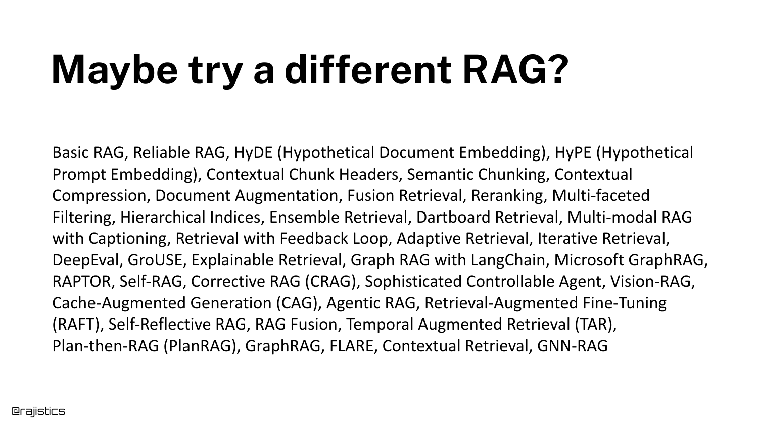
This slide lists a dizzying array of RAG variants (GraphRAG, RAPTOR, CRAG, etc.) and retrieval techniques. It represents the “analysis paralysis” developers face when scouring arXiv papers for a solution to their accuracy problems.
Shah warns against blindly chasing the latest academic paper to fix fundamental system issues. “The answer is not in here of pulling together like a bunch of archive papers.” Instead, he advocates for a structured framework to make decisions.
7. Ultimate RAG Solution
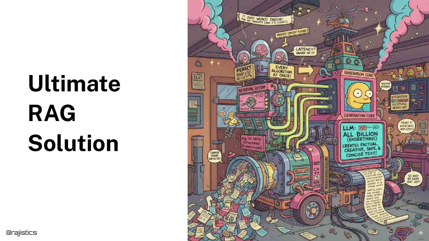
A humorous cartoon depicts a “Rube Goldberg” machine, representing the “Ultimate RAG Solution.” It mocks the tendency to over-engineer systems with too many interconnected, fragile components in the pursuit of performance.
The speaker uses this visual to argue for simplicity and deliberate design. The goal is to avoid building a monstrosity that is impossible to maintain, urging the audience to think about trade-offs before complexity.
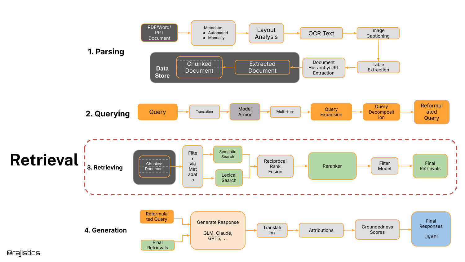
8. RAG as a system
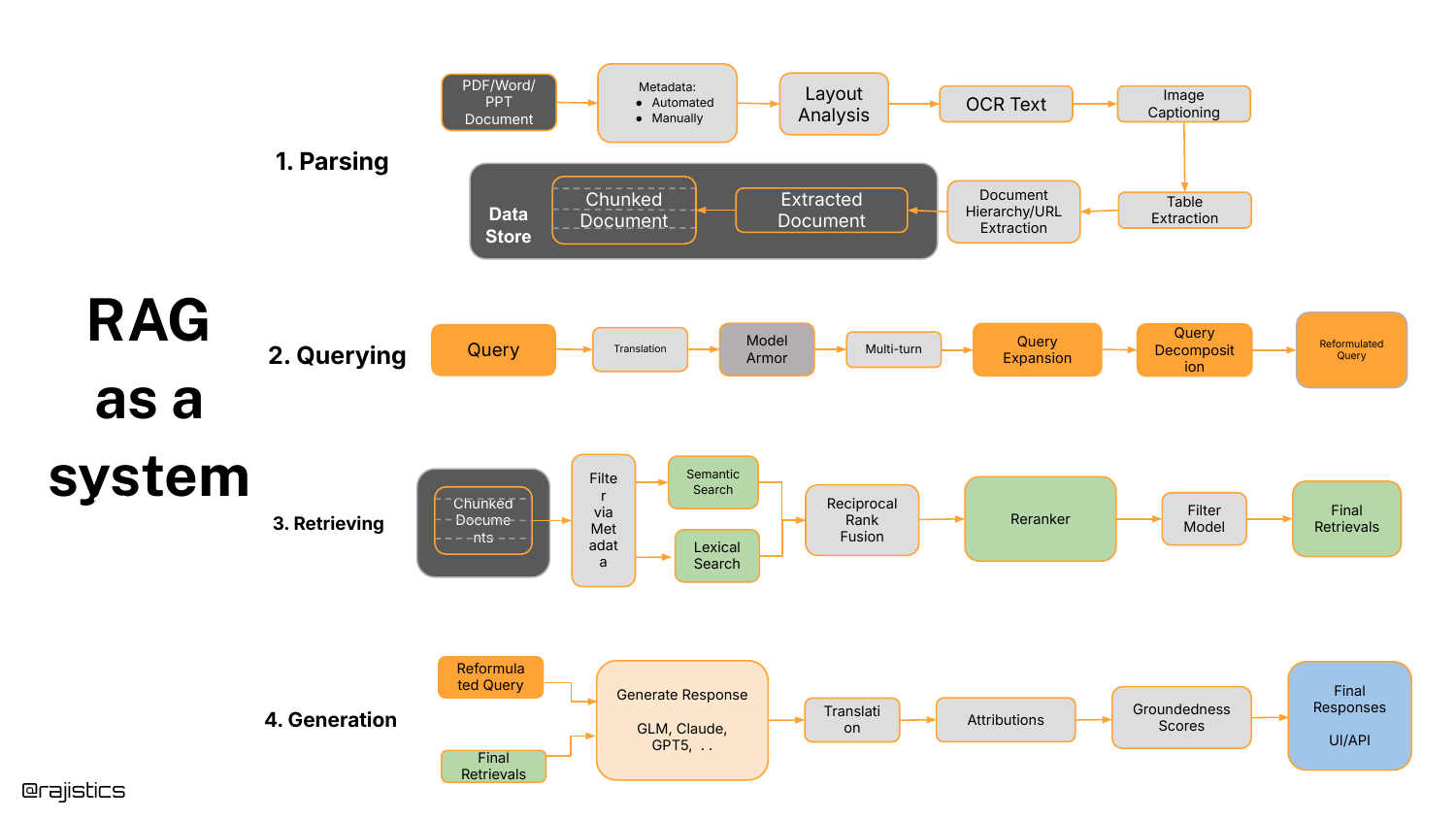
The speaker introduces a clean system architecture for RAG, broken into four distinct stages: Parsing, Querying, Retrieving, and Generation. This framework serves as the mental map for the rest of the presentation.
He highlights that “Parsing” is vastly overlooked—getting information out of complex documents cleanly is a prerequisite for success. Today’s talk, however, will zoom in specifically on the Retrieving and Querying components.
9. Designing a RAG Solution
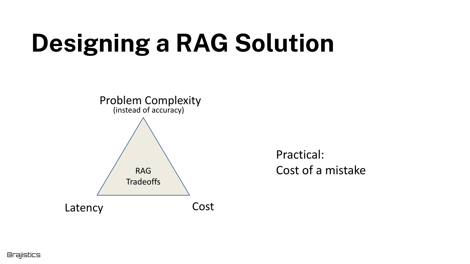
This slide presents a “Tradeoff Triangle” for RAG, balancing Problem Complexity, Latency, and Cost. The speaker advises having a serious conversation with stakeholders about these constraints before writing code.
A key concept introduced here is the “Cost of a mistake.” In coding assistants, a mistake is low-cost (the developer fixes it). In medical RAG systems, the cost of a mistake is high (life or death), which dictates a completely different architectural approach.
10. RAG Considerations
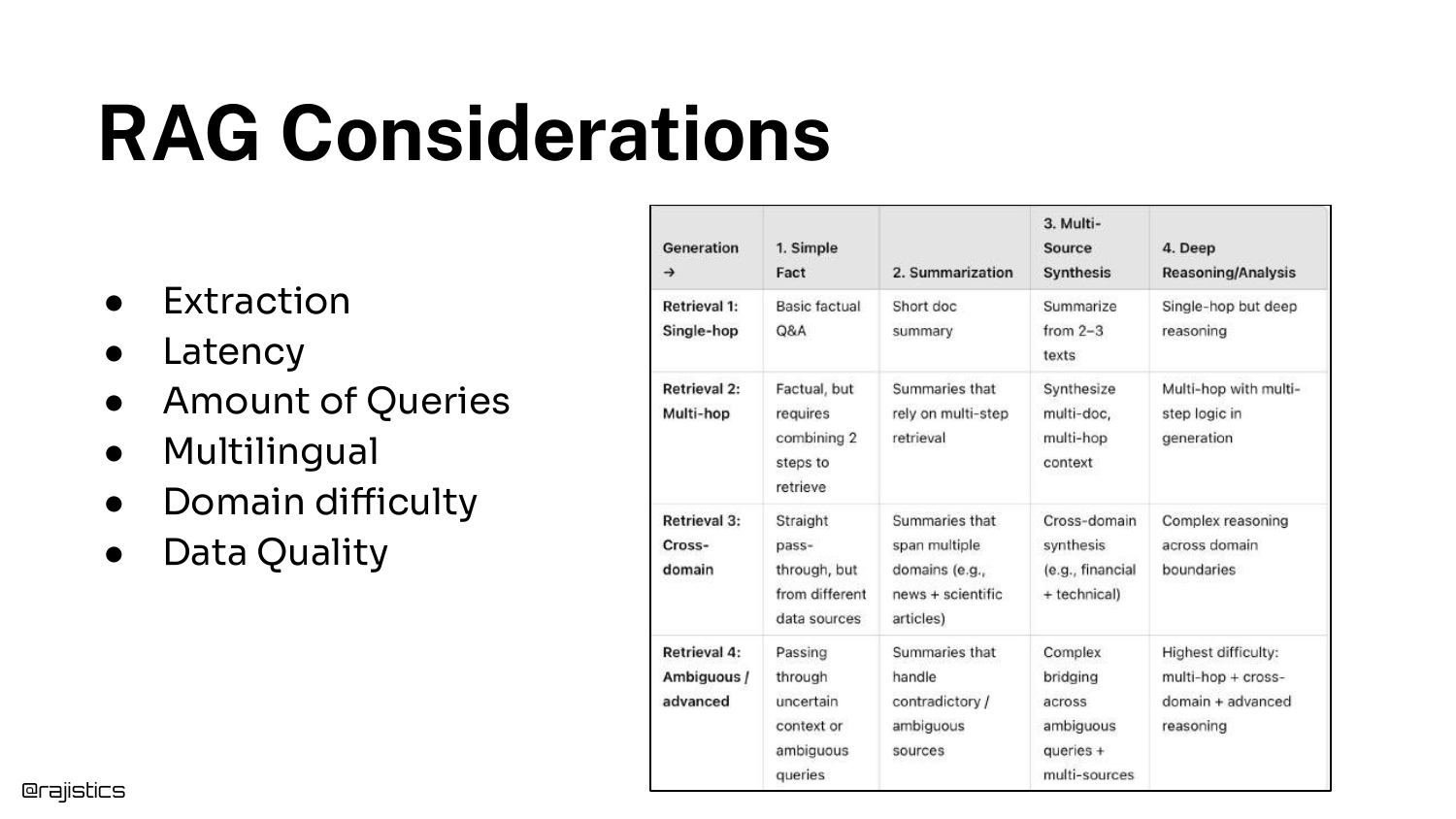
A detailed table breaks down specific considerations that influence RAG design, such as domain difficulty, multilingual requirements, and data quality. This slide was originally created for sales teams to help scope customer problems.
Shah emphasizes that understanding the nuances of the use case upfront saves heartache later. For instance, knowing if users will ask simple questions or require complex reasoning changes the retrieval strategy entirely.
11. Consider Query Complexity
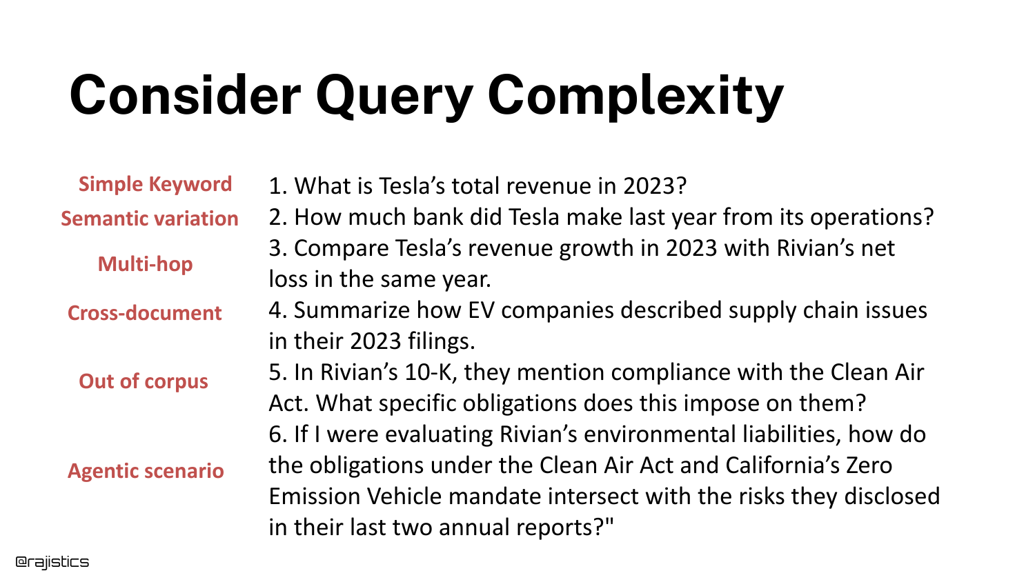
The speaker categorizes queries by complexity, ranging from simple Keywords (“Total Revenue”) to Semantic variations (“How much bank?”), to Multi-hop reasoning, and finally Agentic scenarios.
He points out a common failure mode: “The answers aren’t in the documents… all of a sudden they’re asking for knowledge that’s outside.” Recognizing the query complexity determines whether you need a simple search engine or a complex agentic workflow.
12. Retrieval (Highlighted)
The presentation zooms back into the system diagram, highlighting the “Retrieving” box. This signals the start of the deep technical dive into retrieval algorithms.
Shah notes that this area causes the most confusion due to the sheer number of model choices and architectures available. He aims to provide a practical guide to selecting the right retrieval tool.
13. Retrieval Approaches
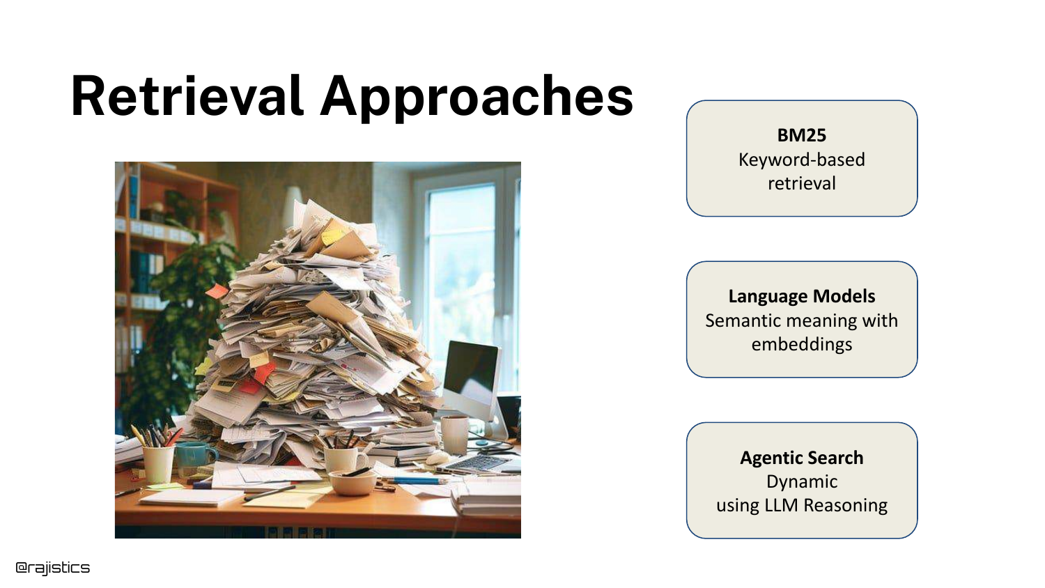
Three primary retrieval pillars are introduced: 1. BM25: The lexical, keyword-based standard. 2. Language Models: Semantic embeddings and vector search. 3. Agentic Search: The new frontier of iterative reasoning.
The speaker emphasizes that documents must be broken into pieces (chunking) because no single model context window is efficient enough to hold all enterprise data for every query.
14. Building RAG is Easy (Code Highlight)
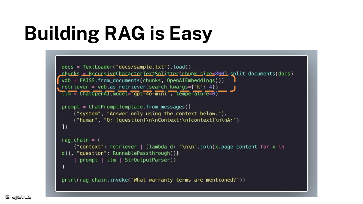
Returning to the initial code snippet, the speaker highlights the vectorstore and retriever initialization lines. This pinpoints exactly where the upcoming concepts fit into the implementation.
This visual anchor helps developers map the theoretical concepts of BM25 and Embeddings back to the actual lines of code they write in libraries like LangChain or LlamaIndex.
15. BM25
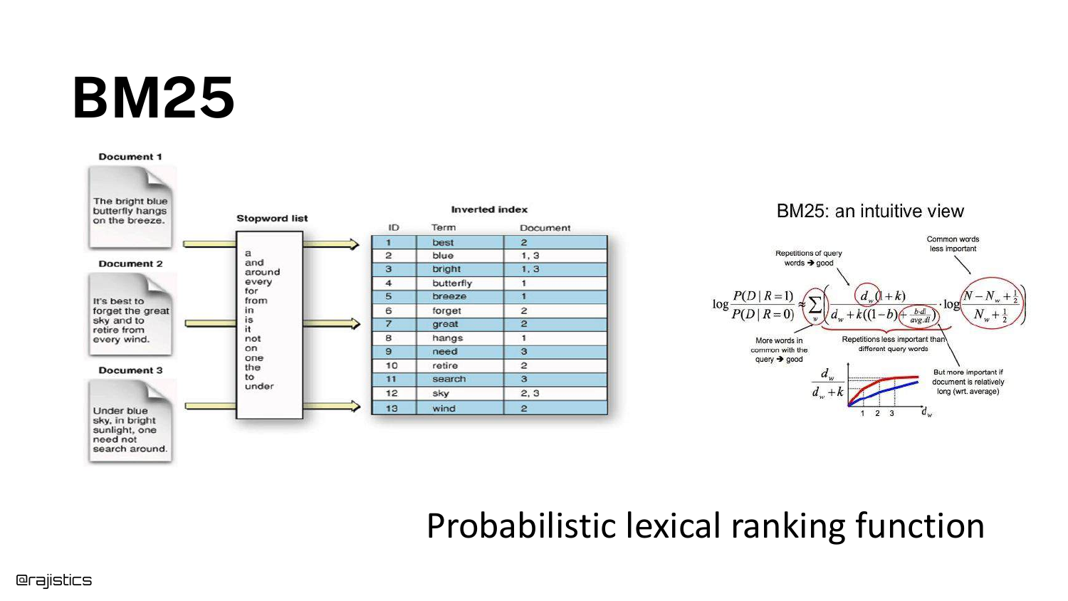
BM25 (Best Match 25) is explained as a probabilistic lexical ranking function. The slide visualizes an inverted index, mapping words (like “butterfly”) to the specific documents containing them.
Shah explains that this is the 25th iteration of the formula, designed to score documents based on word frequency and saturation. It remains a powerful, fast baseline for retrieval.
16. BM25 Performance
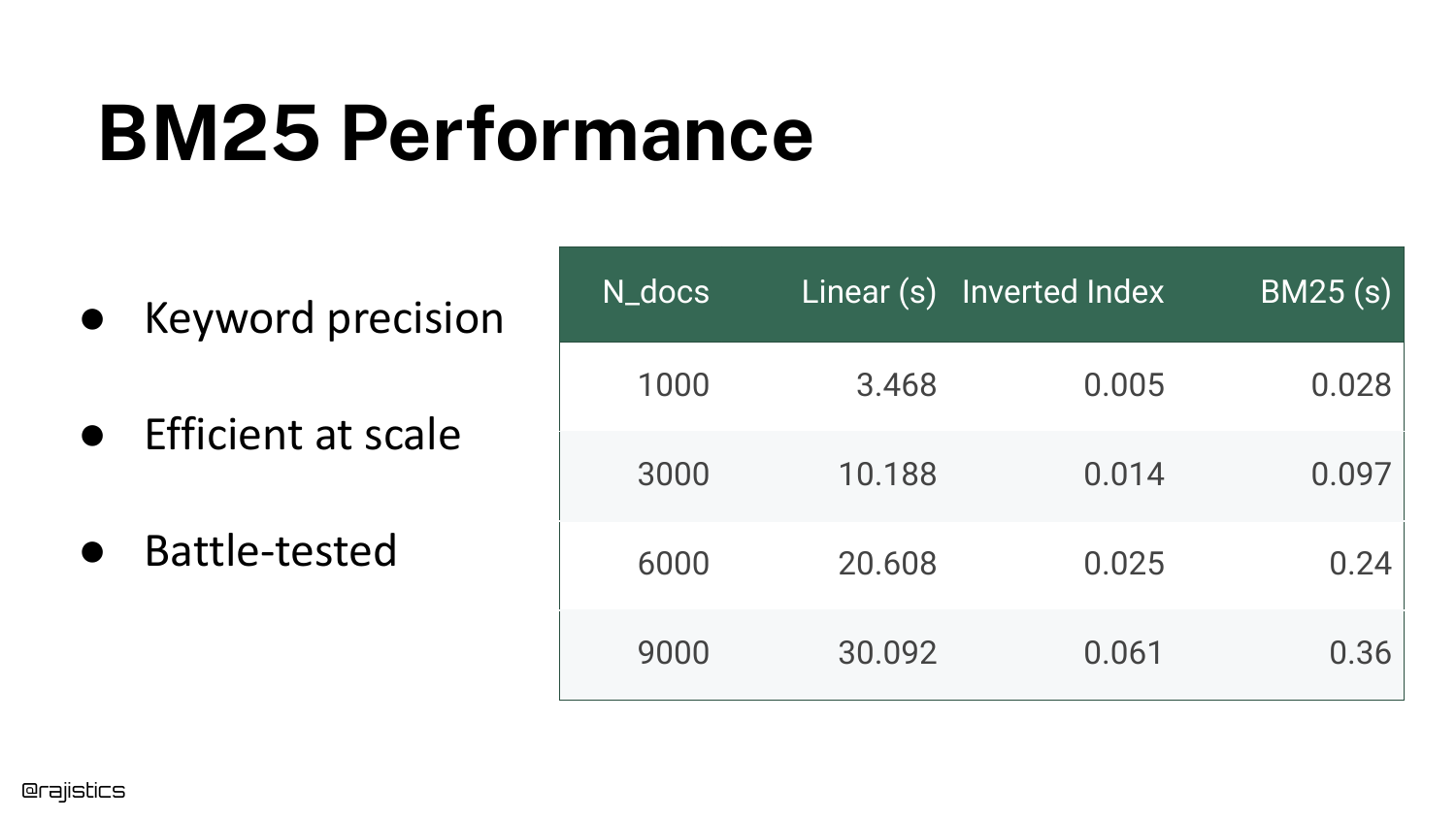
A table compares the speed of a Linear Scan (Ctrl+F style) versus an Inverted Index (BM25) as the document count grows from 1,000 to 9,000.
The data shows that linear search becomes exponentially slower (taking 3,000 seconds for 1k documents in this synthetic test), while BM25 remains orders of magnitude faster. This efficiency is why lexical search is still widely used in production.
17. BM25 Failure Cases
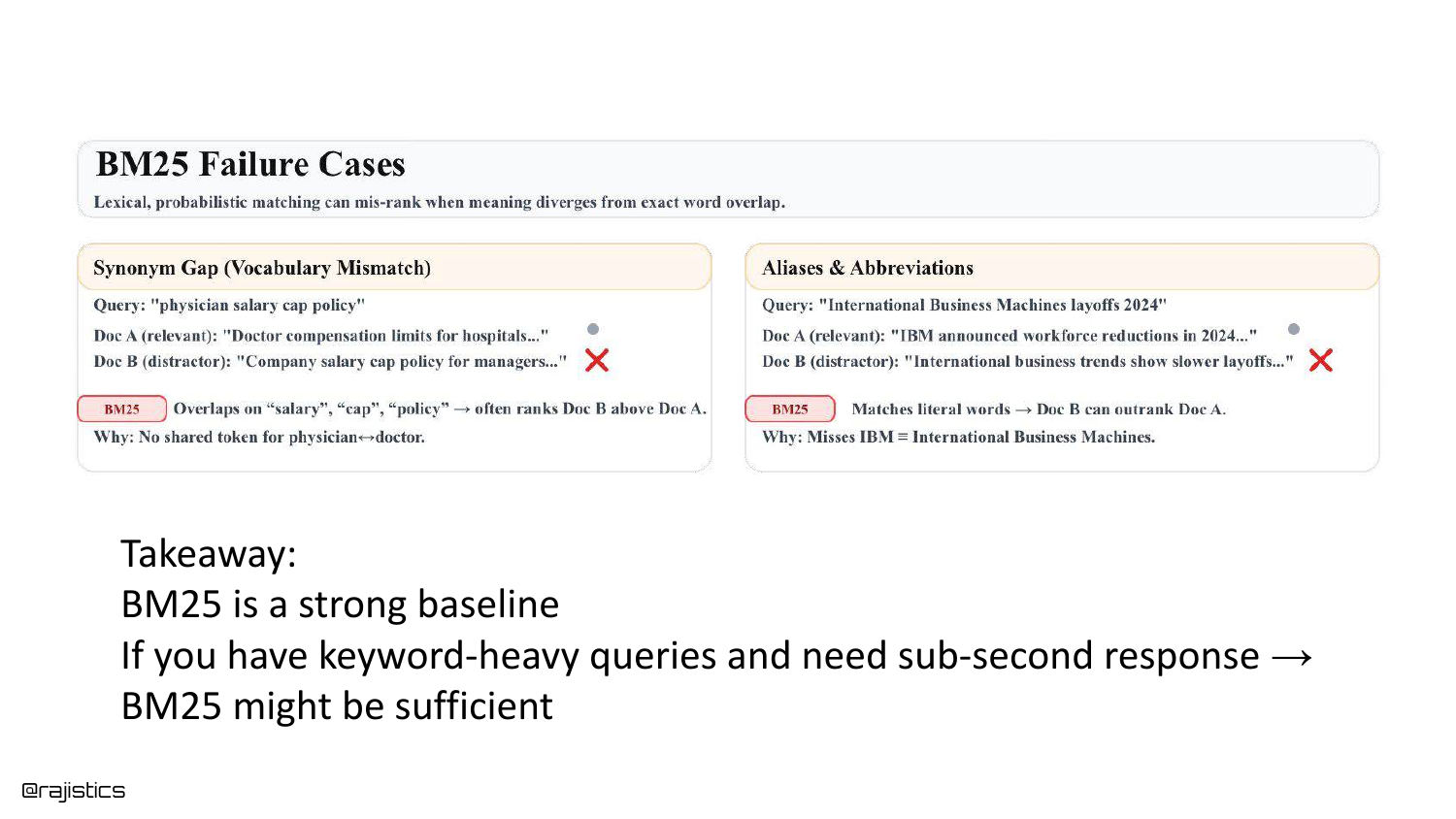
The limitations of BM25 are exposed. Because it relies on exact word matches, it fails when users use synonyms. If a user searches for “Physician” but the documents only contain “Doctor,” BM25 will return zero results.
Similarly, it struggles with acronyms like “IBM” vs “International Business Machines.” Despite this, Shah argues BM25 is a “very strong baseline” that often beats complex neural models on specific keyword-heavy datasets.
18. Hands on: BM25s
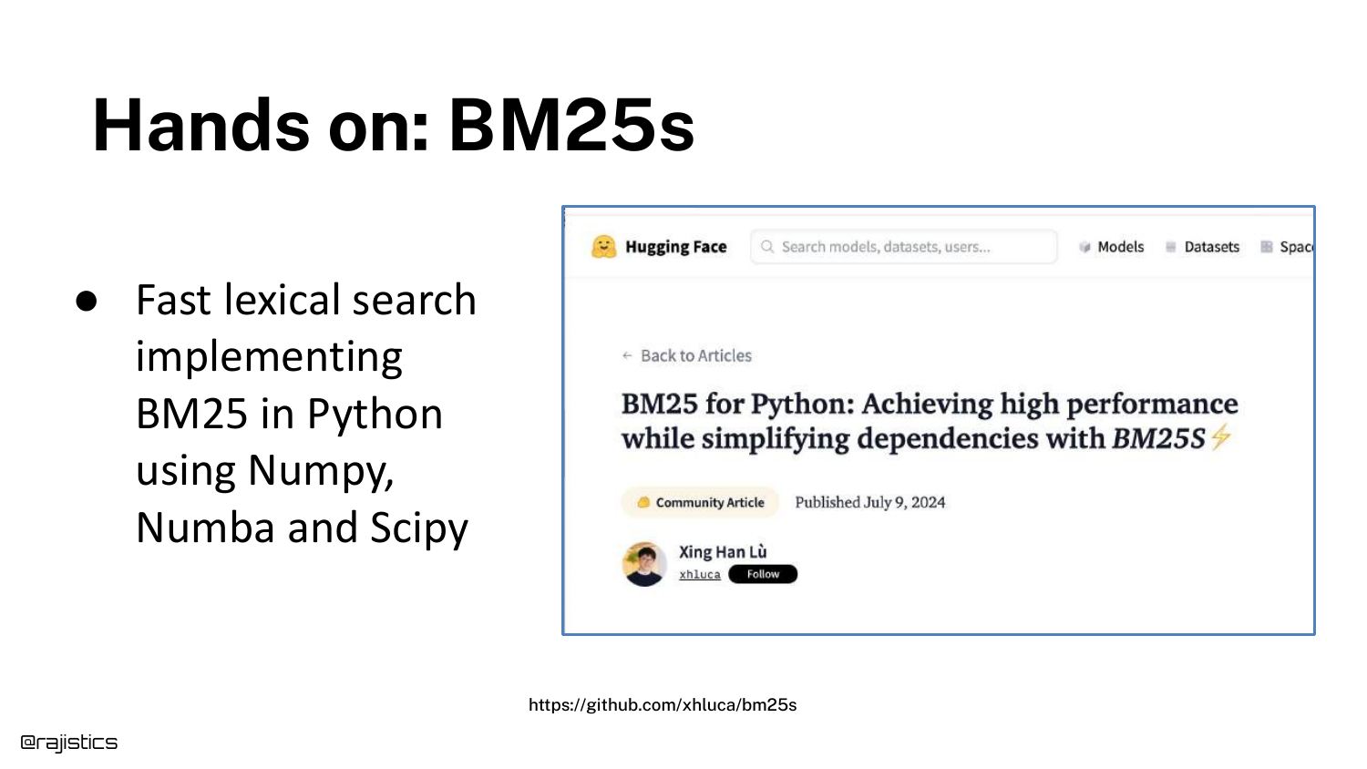
For developers wanting to implement this, the slide points to a library called bm25s, a high-performance Python implementation available on Hugging Face.
This reinforces the practical nature of the talk—BM25 isn’t just a legacy concept; it is an active, installable tool that developers should consider using alongside vector search.
19. Enter Language Models
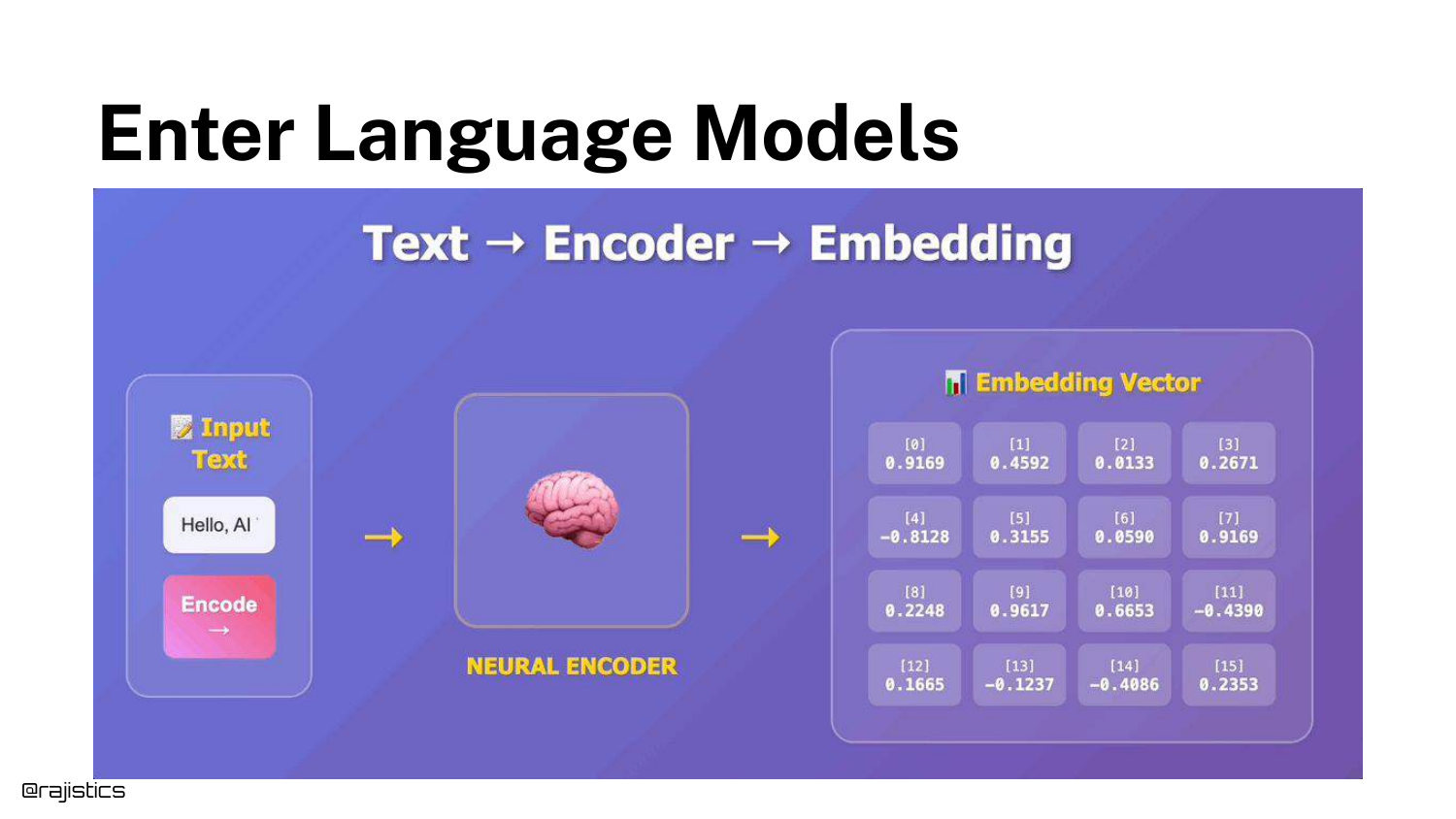
The talk transitions to Language Models (Embeddings). The slide explains how an encoder model turns text into a dense vector (a list of numbers) that captures semantic meaning.
Because these models are trained on vast amounts of data, they “have an idea of these similar concepts.” This solves the synonym problem that plagues BM25.
20. Embeddings Visualized
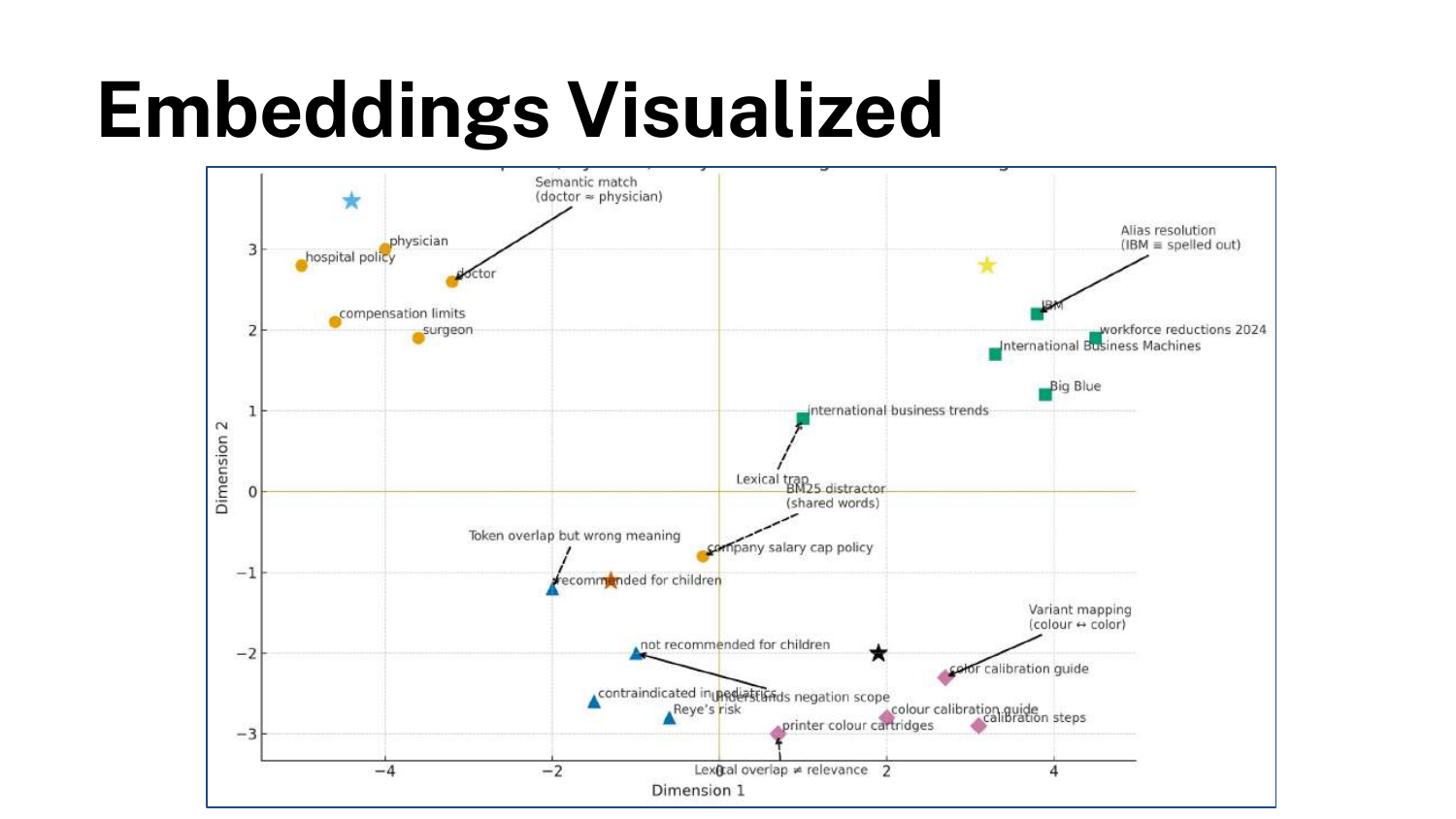
A 2D visualization demonstrates how embeddings group related concepts in latent space. The word “Doctor” and “Physician” would be located very close to each other mathematically.
This spatial proximity allows for Semantic Search: finding documents that mean the same thing as the query, even if they don’t share a single word.
21. Semantic search is widely used
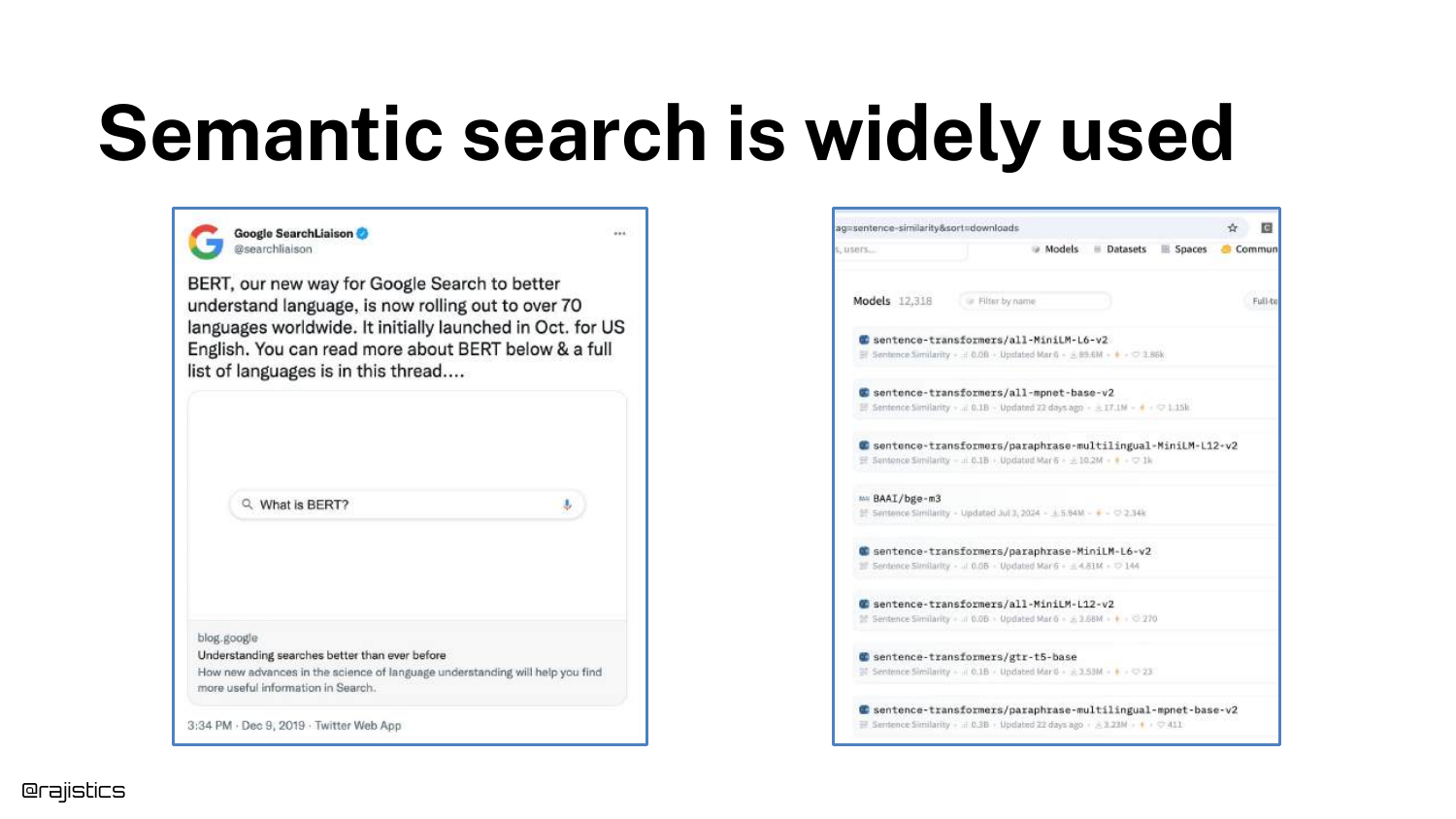
The speaker validates the importance of semantic search by showing a tweet from Google’s SearchLiaison regarding BERT, and a screenshot of Hugging Face’s model repository.
This confirms that semantic search is the industry standard for modern information retrieval, having been deployed at massive scale by tech giants to improve result relevance.
22. Which language model?
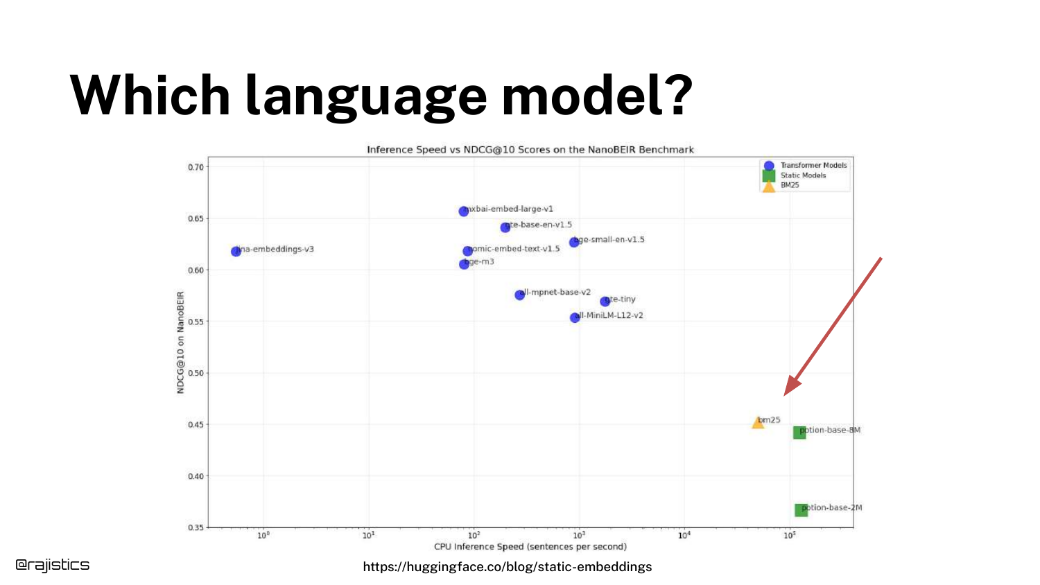
A scatter plot compares various models based on Inference Speed (X-axis) and NDCG@10 (Y-axis, a measure of retrieval quality).
Shah places BM25 on the right (fast but lower accuracy) to orient the audience. He points out that there is a massive variety of models with different trade-offs between compute cost and retrieval quality.
23. Static Embeddings
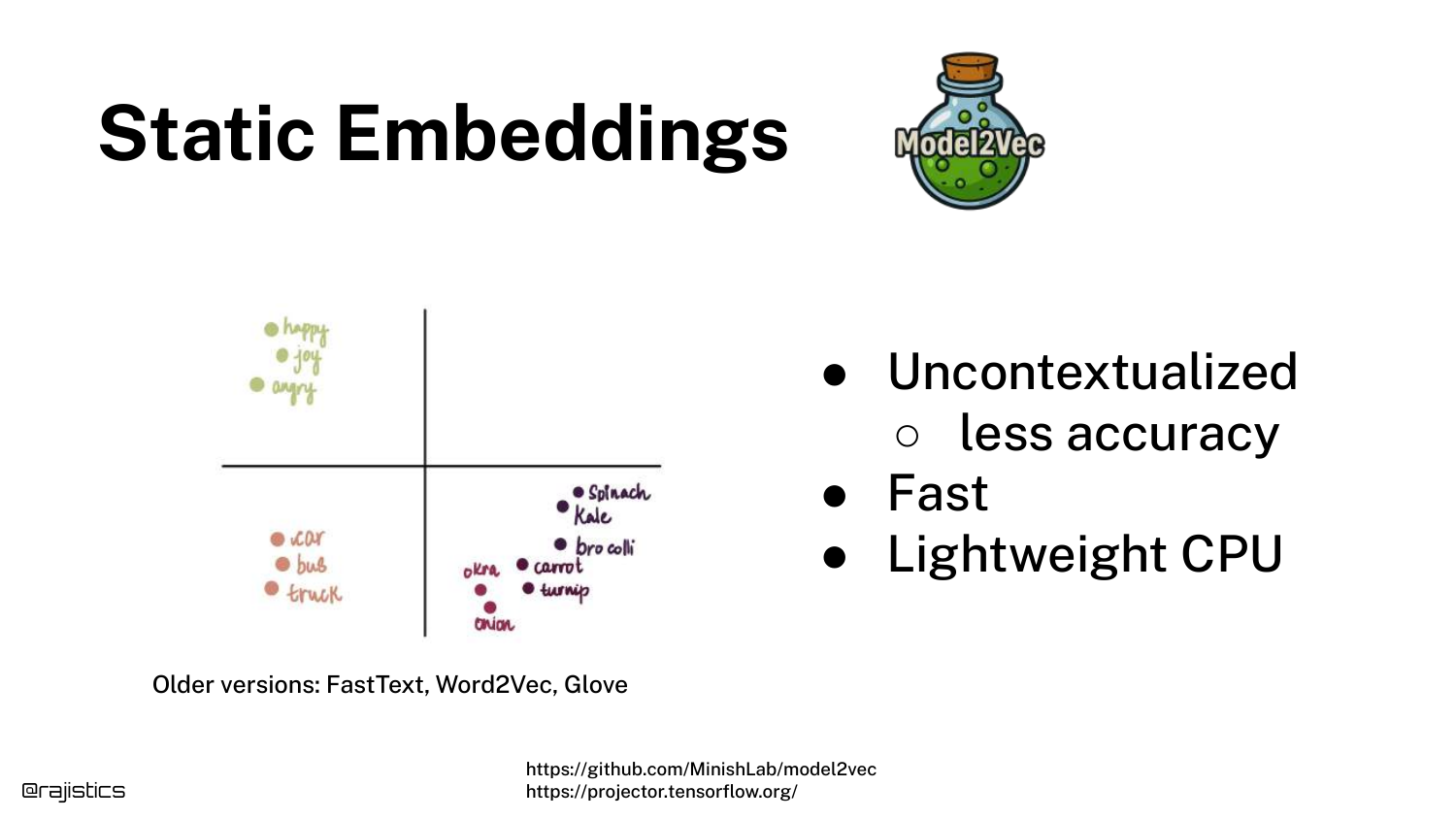
The speaker introduces Static Embeddings (like Word2Vec or GloVe) which are located on the far right of the previous scatter plot—extremely fast, even on CPUs.
These models assign a fixed vector to every word. While efficient, they lack context. The word “bank” has the same vector whether referring to a river bank or a financial bank, which limits their accuracy.
24. Why Context Matters
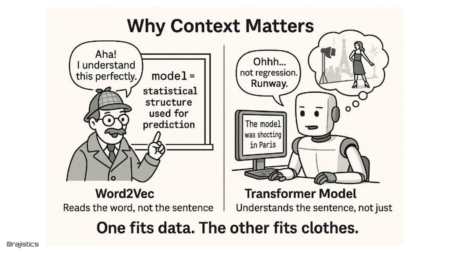
A cartoon illustrates the difference between Static Embeddings and Transformers. The Transformer can distinguish between “Model” in a data science context versus “Model” in a fashion context.
This contextual awareness is why modern Transformer-based embeddings (like BERT) generally outperform static embeddings and BM25 in complex retrieval tasks, despite being slower.
25. Many more models!
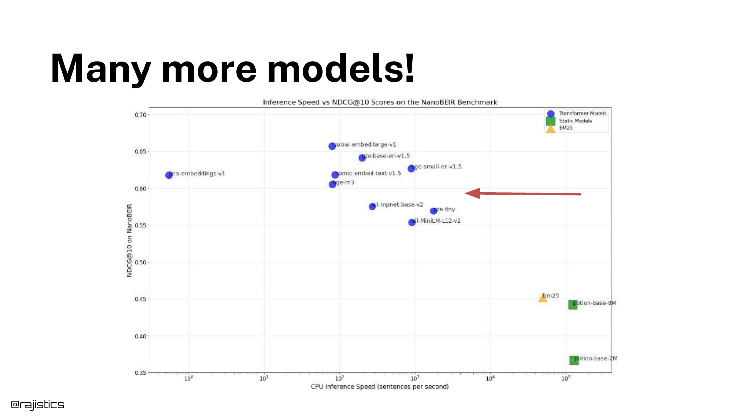
Returning to the scatter plot, a red arrow points toward the top-left quadrant—models that are slower but achieve higher accuracy.
The speaker notes that the field is constantly evolving, with “newer generations of models” pushing the boundary of what is possible in terms of retrieval quality.
26. MTEB/RTEB
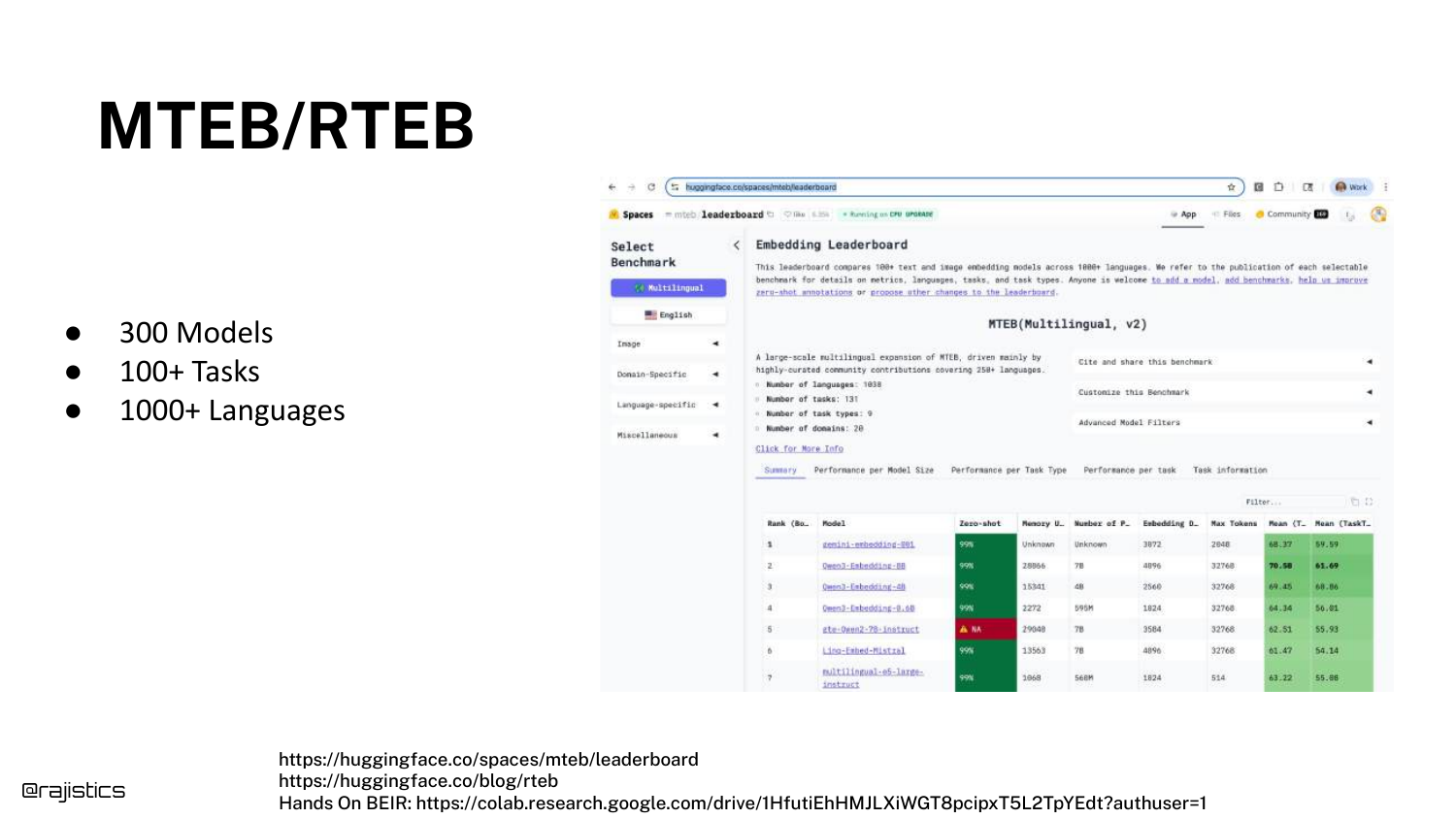
To help developers choose, Shah introduces the MTEB (Massive Text Embedding Benchmark) and RTEB (Retrieval Text Embedding Benchmark). These are leaderboards hosted on Hugging Face.
He highlights a key distinction: MTEB uses public datasets, while RTEB uses private, held-out datasets. This is crucial for avoiding “data contamination,” where models perform well simply because they were trained on the test data.
27. Selecting an embedding model
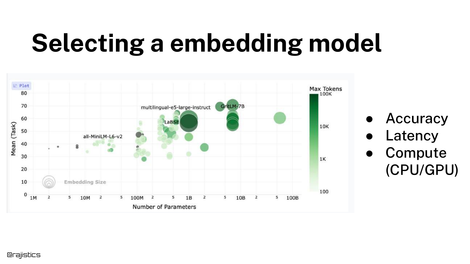
The speaker switches to a live browser view (captured in the slide) of the leaderboard. He discusses the bubble chart visualization where size often correlates with parameter count.
He points out an interesting trend: “You’ll see that there’s a bunch of models here that are all the same size… but the performance differs.” This indicates improvements in training strategies and architecture rather than just throwing more compute at the problem.
28. Selecting an embedding model (Other Considerations)
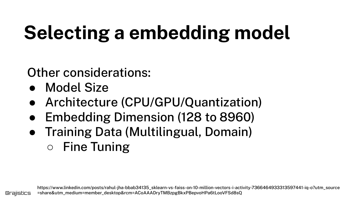
Beyond the leaderboard score, Shah lists practical selection criteria: Model Size (can it fit in memory?), Architecture (CPU vs GPU), Embedding Dimension (storage costs), and Training Data (multilingual support).
He advises checking if a model is open source and quantizable, as this can significantly reduce latency without a major hit to accuracy.
29. Matryoshka Embedding Models
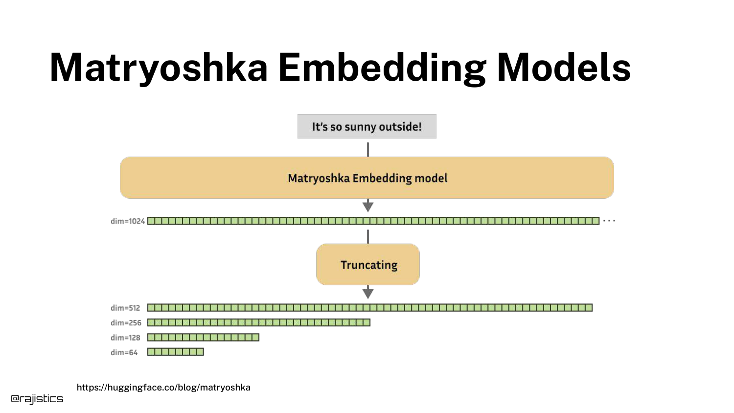
A specific innovation is highlighted: Matryoshka Embeddings. These models allow developers to truncate vectors (e.g., from 768 dimensions down to 64) while retaining most of the performance.
This is a “neat kind of innovation” for optimizing storage and search speed. OpenAI’s newer models also support this feature, offering flexibility between cost and accuracy.
30. Sentence Transformer
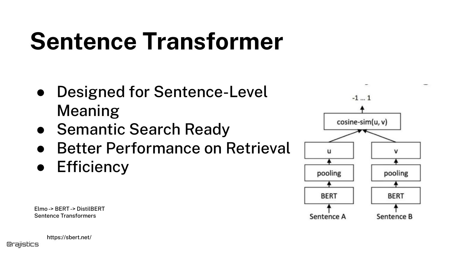
The Sentence Transformer architecture is described as the dominant approach for RAG. Unlike standard BERT which works on tokens, these are fine-tuned to understand full sentences and paragraphs.
This architecture uses Siamese networks to ensure that semantically similar sentences are close in vector space, making them ideal for the “chunk-level” retrieval required in RAG.
31. Cross Encoder / Reranker

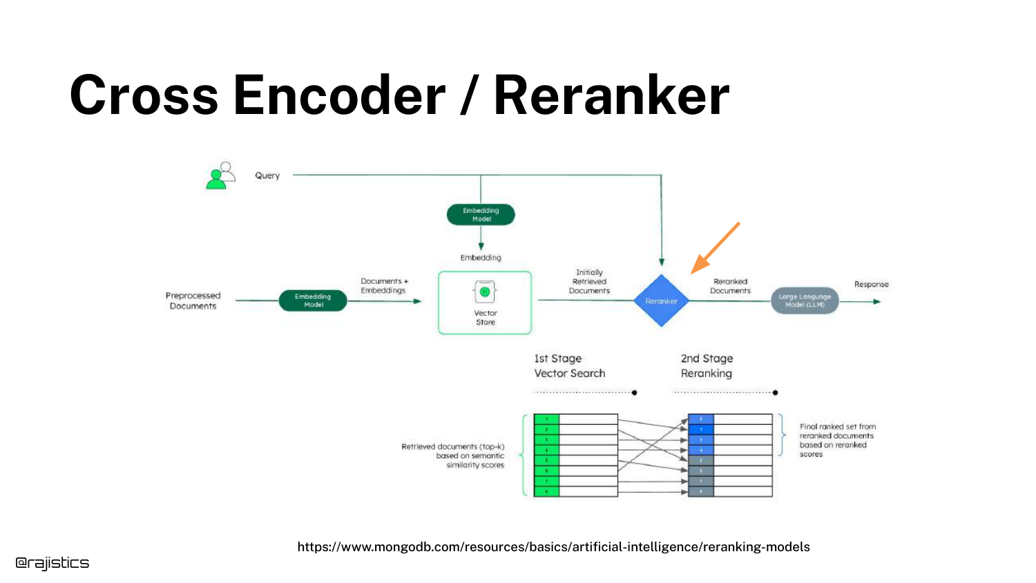
The concept of a Cross Encoder (or Reranker) is introduced. Unlike the bi-encoder (retriever) which processes query and document separately, the cross-encoder processes them together.
This allows for a much deeper calculation of relevance. It is typically used as a second stage: retrieve 50 documents quickly with vectors, then use the slow but accurate Cross Encoder to rank the top 5.
32. Cross Encoder / Reranker (Duplicate)
(This slide reinforces the previous diagram, emphasizing the “crossing” of the query and document in the model architecture.)
33. Cross Encoder / Reranker (Accuracy Boost)
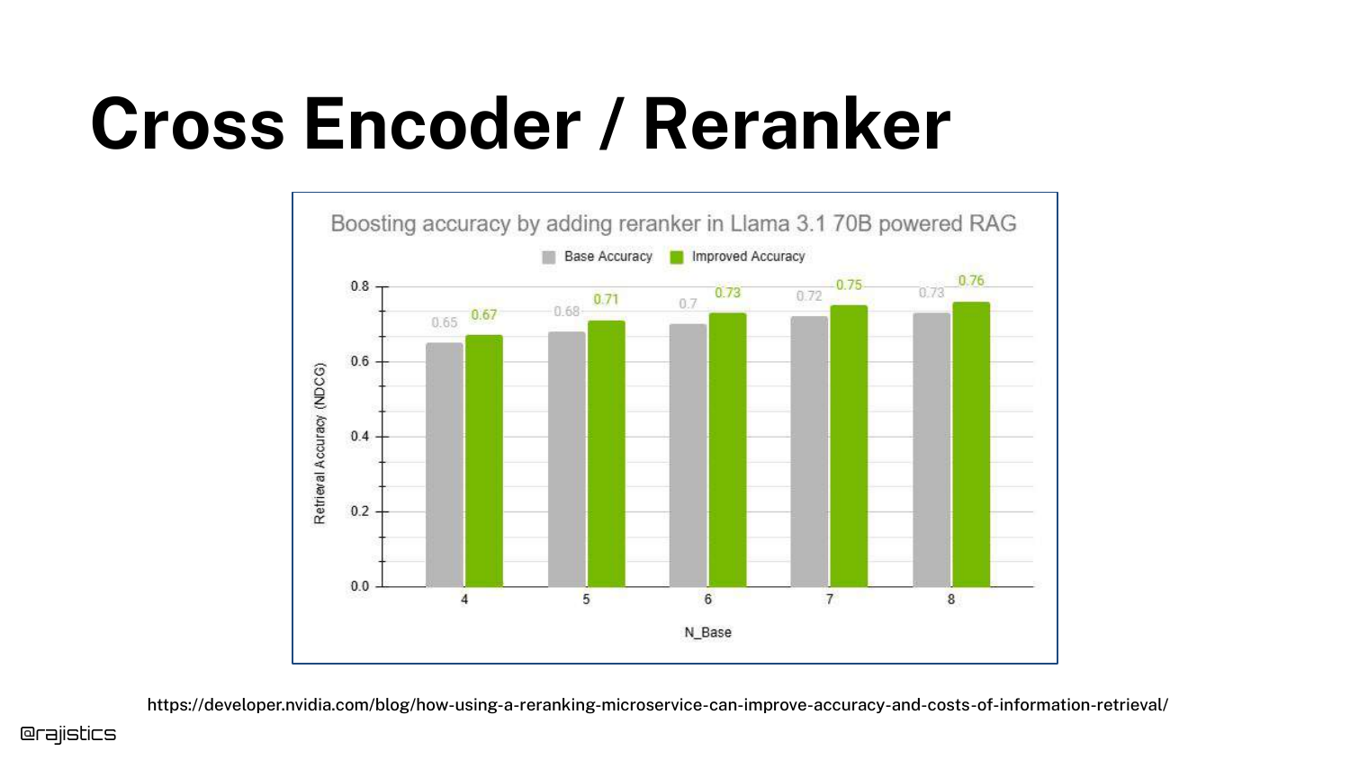
A bar chart quantifies the value of reranking. It shows a significant boost in NDCG (accuracy) when a reranker is added to the pipeline.
The speaker notes that while you get a “bump” in quality, it “doesn’t come for free.” The trade-off is increased latency, as the cross-encoder is computationally expensive.
34. Cross Encoder / Reranker (Execution Flow)
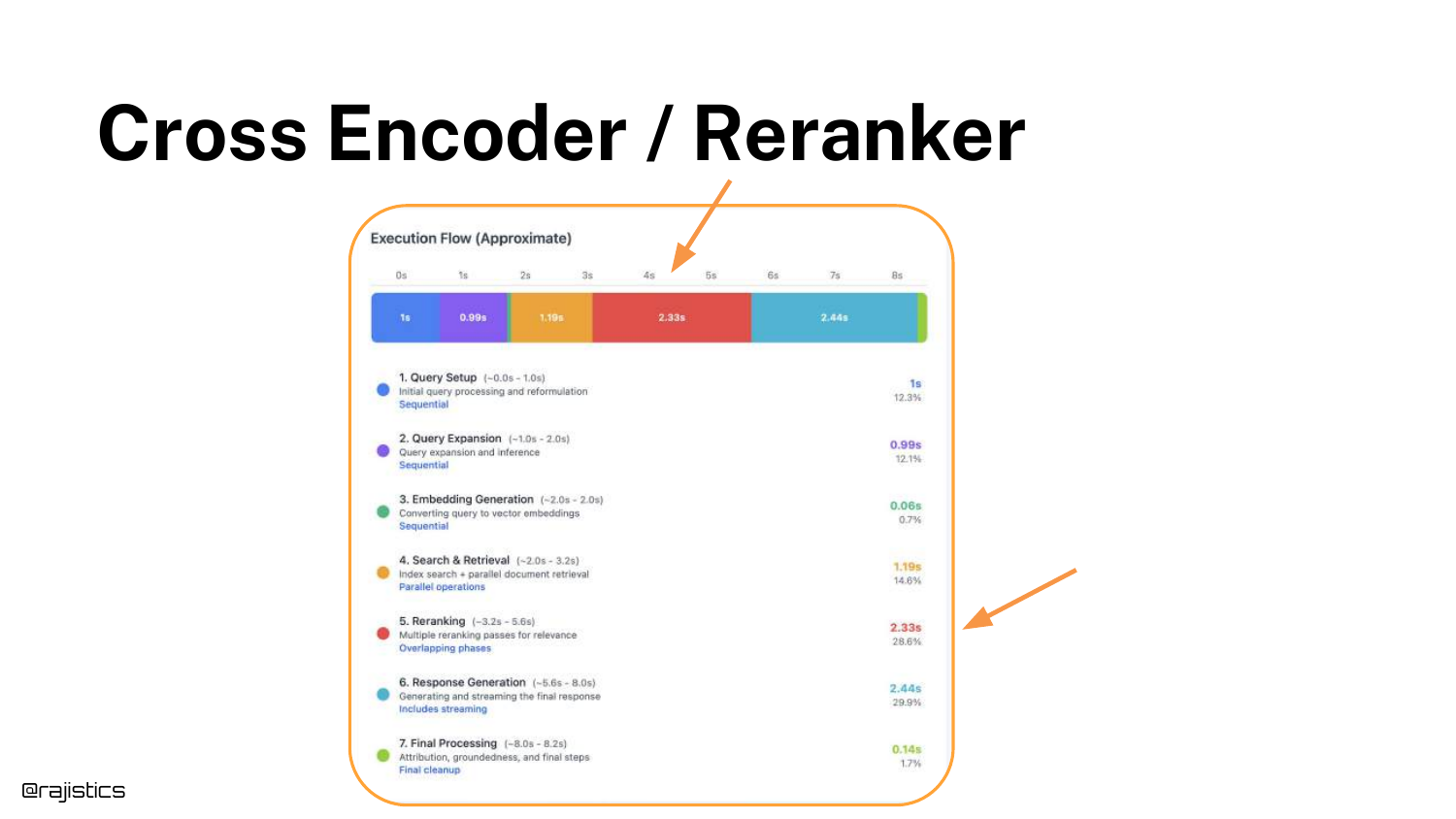
The execution flow diagram highlights the reranker’s position in the pipeline. It sits between the Vector Store retrieval and the LLM generation.
This visual reinforces the latency implication: the user has to wait for both the initial search and the reranking pass before the LLM even starts generating an answer.
35. Hands On: Retriever & Reranker
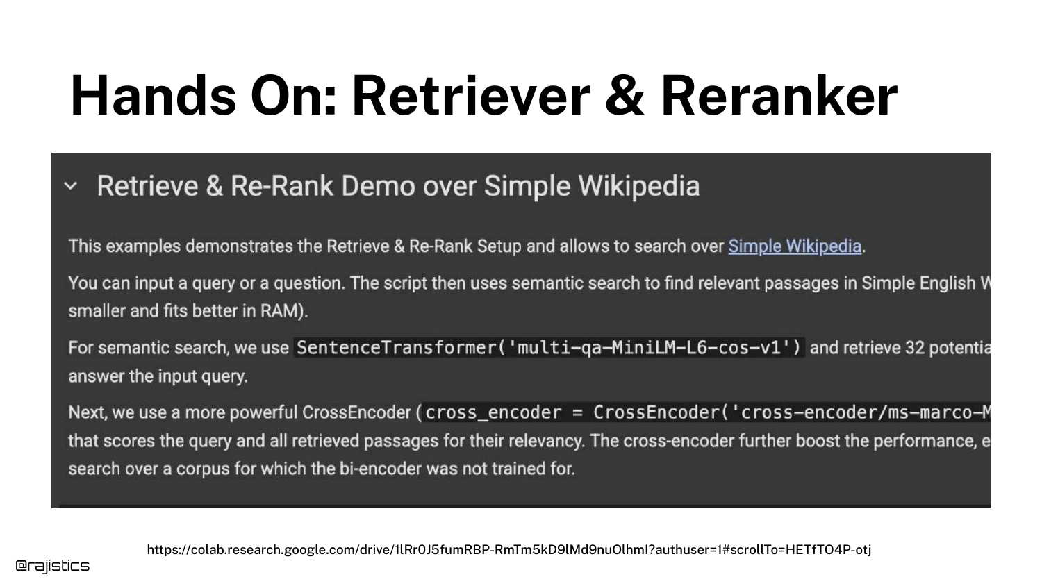
A screenshot of a Google Colab notebook is shown, demonstrating a practical implementation of the Retrieve and Re-rank strategy using the SentenceTransformer and CrossEncoder libraries.
This provides a concrete resource for the audience to test the accuracy vs. speed trade-offs themselves on simple datasets like Wikipedia.
36. Instruction Following Reranker
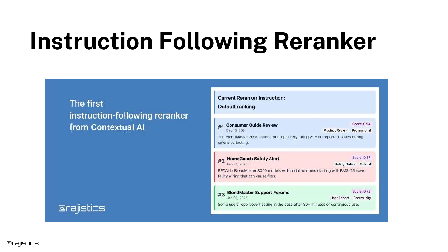
Shah mentions a specific advancement: Instruction Following Rerankers (developed by his company, Contextual). These allow developers to pass a prompt to the reranker, such as “Prioritize safety notices.”
This adds a “knob” for developers to tune retrieval based on business logic without retraining the model.
37. Combine Multiple Retrievers
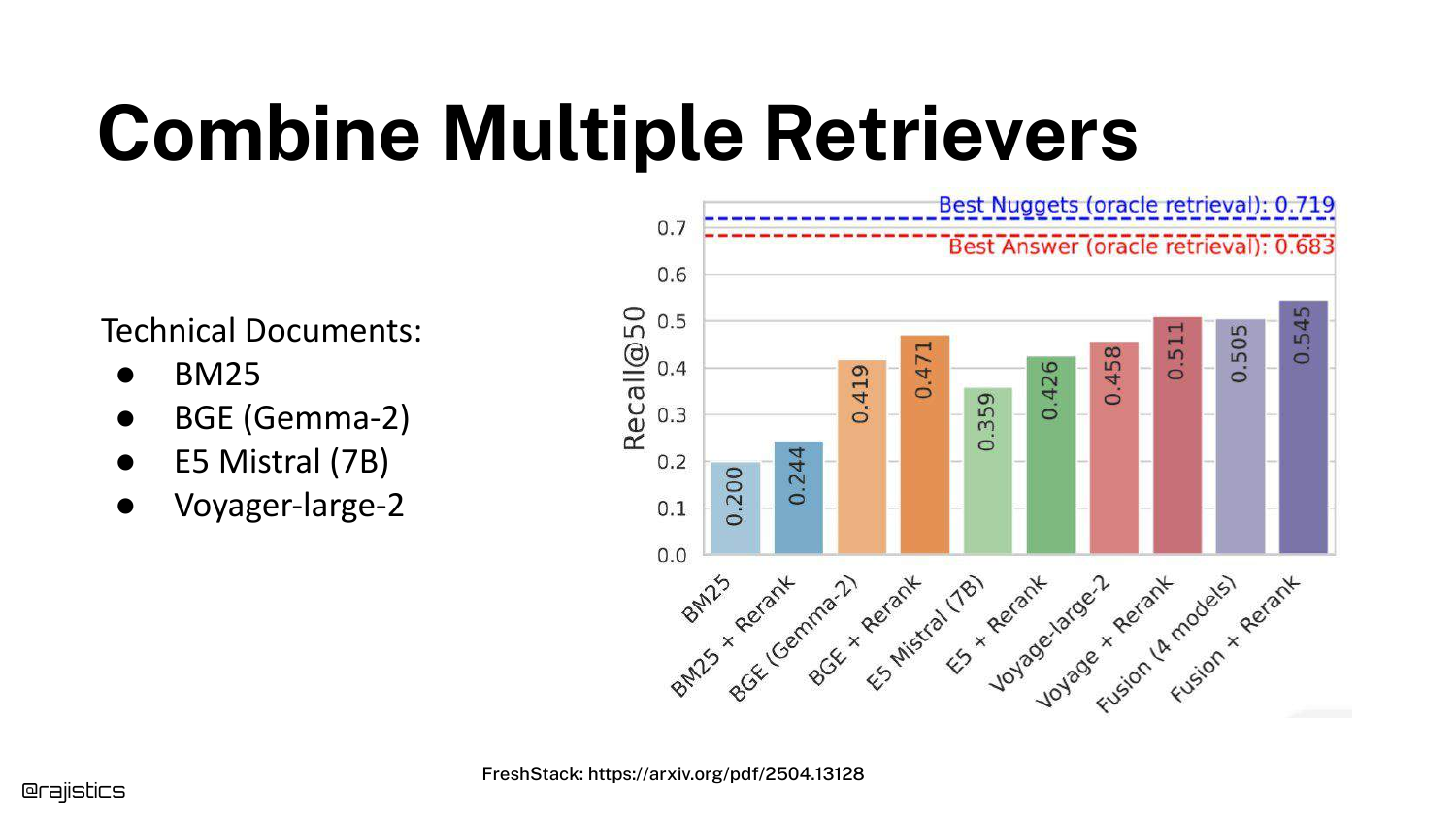
The presentation suggests that you don’t have to pick just one method. You can combine BM25, various embedding models (E5, BGE), and rerankers.
While combining them (Ensemble Retrieval) often yields better recall, Shah warns that “you got to engineer this.” Managing multiple indexes and fusion logic increases operational complexity and compute costs.
38. Cascading Rerankers in Kaggle
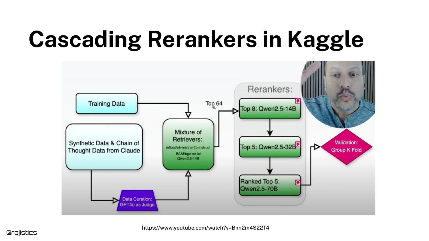
A complex diagram from a Kaggle competition winner illustrates a Cascade Strategy. The solution used three different rerankers, filtering from 64 documents down to 8, and then to 5.
This shows the extreme end of retrieval engineering, where multiple models are chained to squeeze out every percentage point of accuracy.
39. Best practices
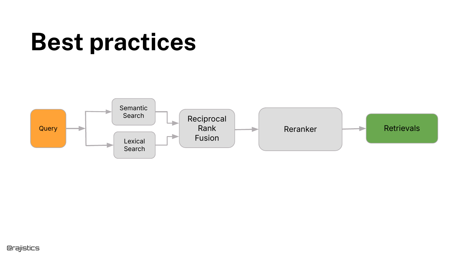
Shah distills the complexity into a recommended Best Practice: 1. Hybrid Search: Combine Semantic Search (Vectors) and Lexical Search (BM25). 2. Reciprocal Rank Fusion: Merge the results. 3. Reranker: Pass the top results through a cross-encoder.
This setup provides a “pretty good standard performance out of the box” and should be the default baseline before trying exotic methods.
40. Families of Embedding Models
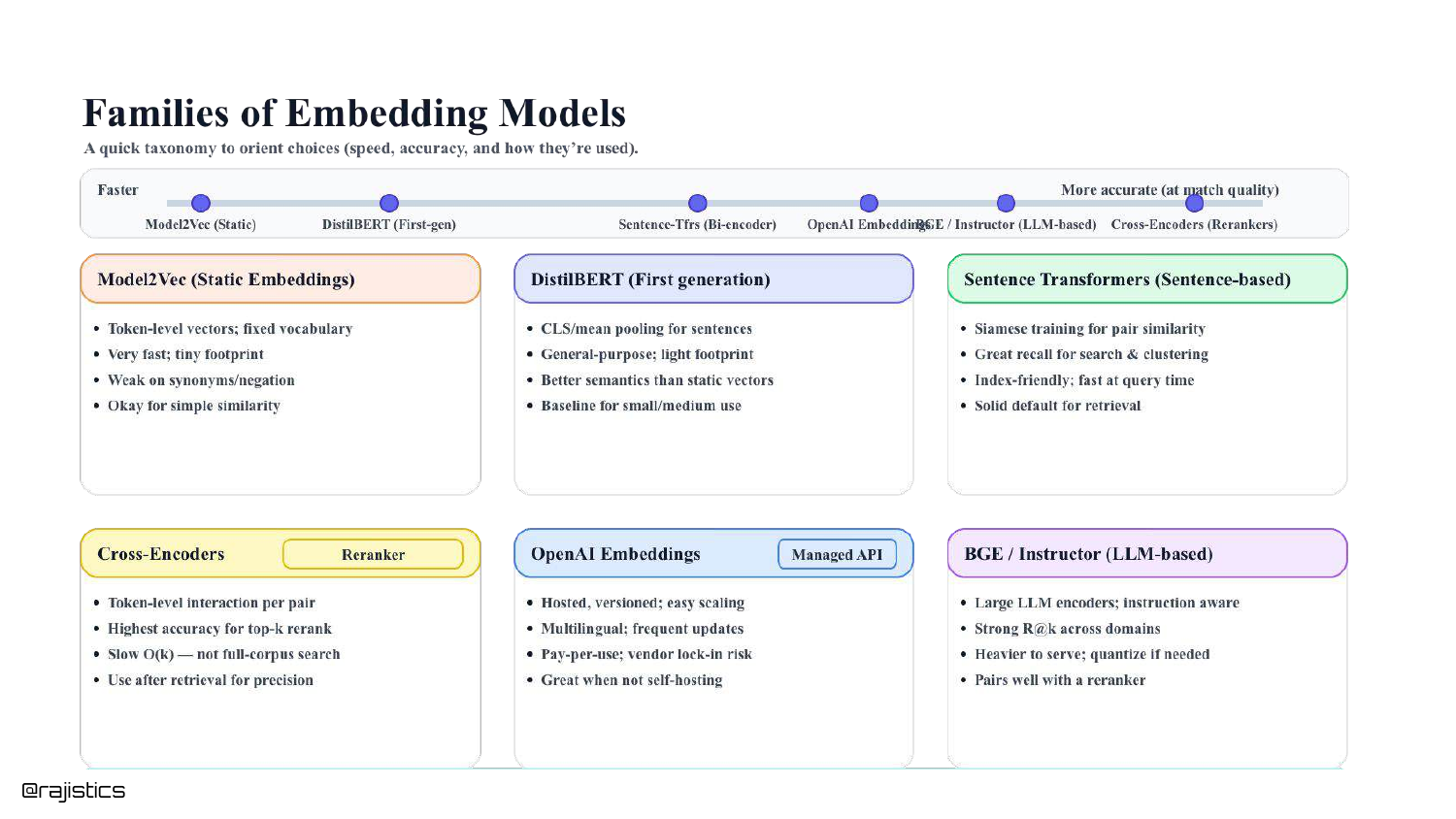
A taxonomy slide categorizes the models discussed: Static (Fastest/Low Accuracy), Bi-Encoders (Fast/Good Accuracy), and Cross-Encoders (Slow/Best Accuracy).
This summary helps the audience mentally organize the tools available in their toolbox.
41. Lots of New Models
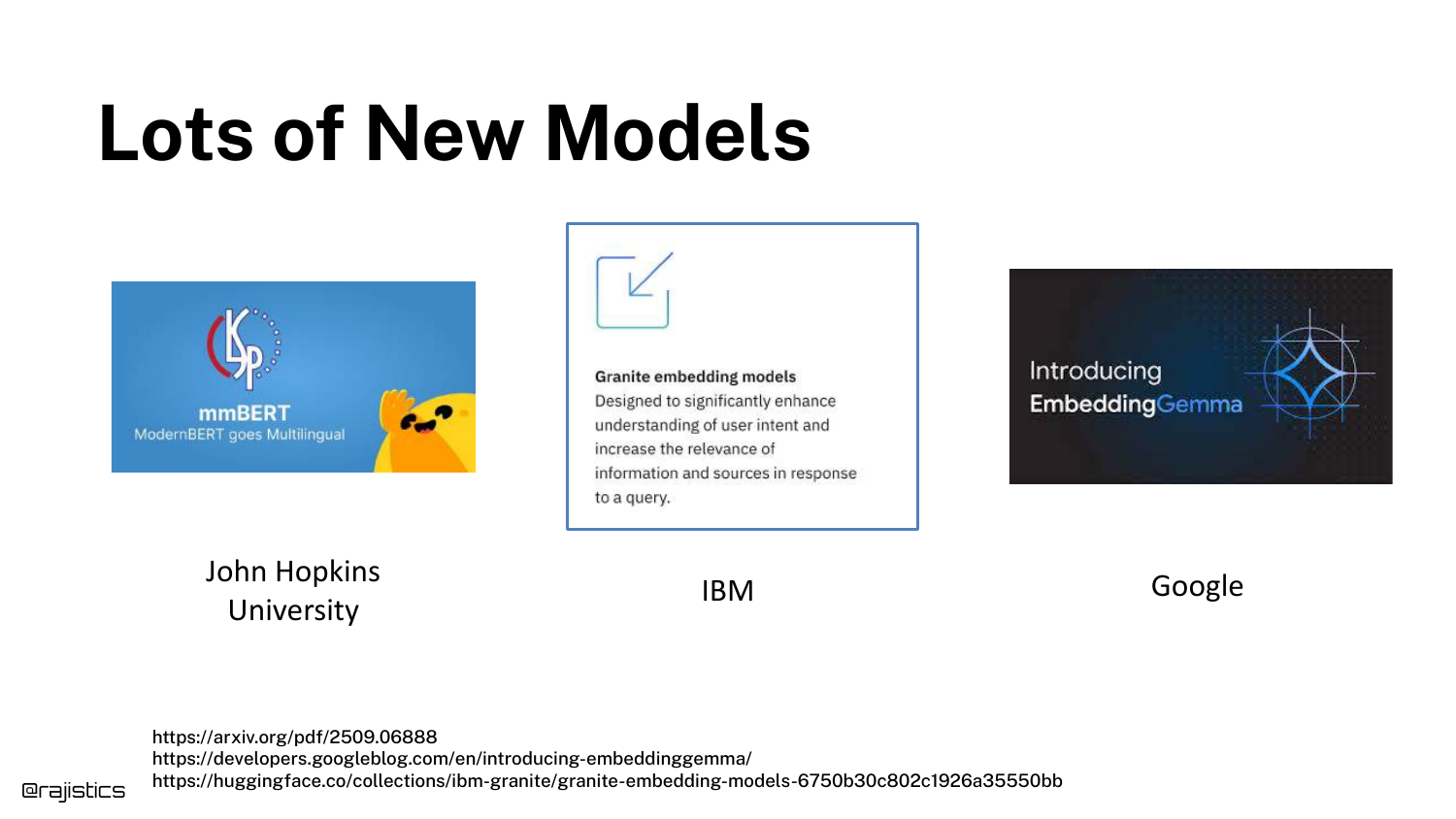
Logos for IBM Granite, Google EmbeddingGemma, and others appear. The speaker notes that while new models from major players appear weekly, the improvements are often “incremental.”
He advises against “ripping up” a working system just to switch to a model that is 1% better on a leaderboard.
42. Other retrieval methods
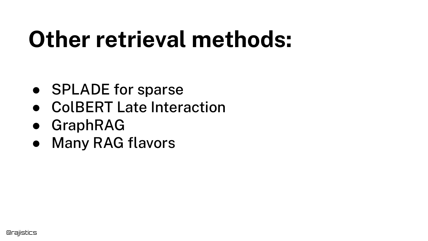
Alternative methods are briefly listed: SPLADE (Sparse retrieval), ColBERT (Late interaction), and GraphRAG.
Shah acknowledges these exist and may fit specific niches, but warns against chasing the “flavor of the week” before establishing a solid baseline with hybrid search.
43. Operational Concerns
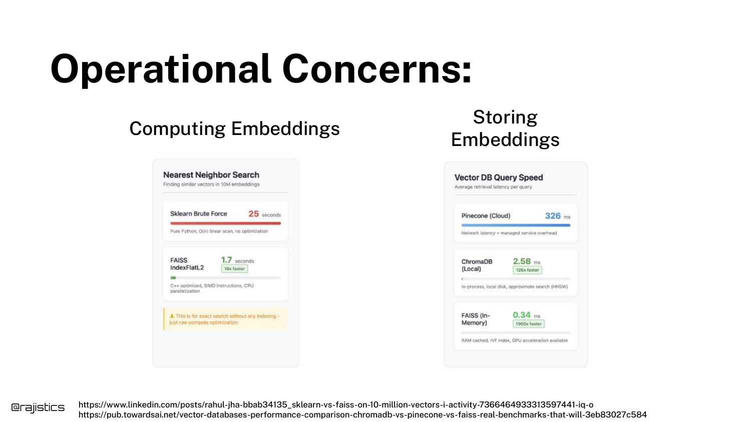
The talk shifts to operations. Libraries like FAISS are mentioned for efficient vector similarity search.
A key point is that for many use cases, you can simply store embeddings in memory. You don’t always need a complex vector database if your dataset fits in RAM.
44. Vector Database Options
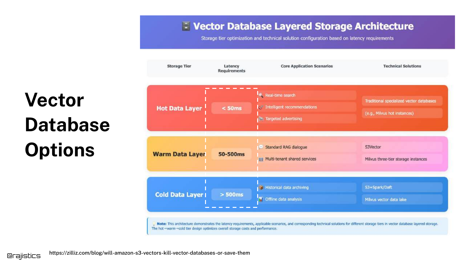
A diagram categorizes storage into Hot (In-Memory), Warm (SSD/Disk), and Cold tiers.
Shah notes there are “tons of vector database options” (Snowflake, Pinecone, etc.). The choice should be governed by latency requirements. If you need sub-millisecond retrieval, you need in-memory storage.
45. Operational Concerns (Datastore Size)
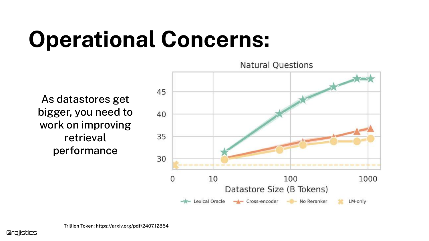
A graph shows that as Datastore Size increases (X-axis), retrieval performance naturally degrades (Y-axis).
To combat this, the speaker strongly recommends using Metadata Filtering. “If you’re not using something like metadata… it’s going to be very tough.” Narrowing the search scope is essential for scaling to millions of documents.
46. Search Strategy Comparison
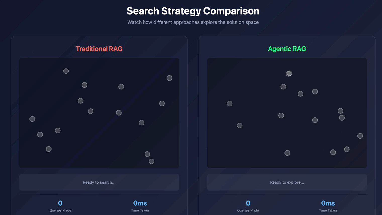
The presentation pivots to the “exciting part”: Agentic RAG. A visual compares “Traditional RAG” (a linear path) with “Agentic RAG” (a winding, exploratory path).
This represents the shift from a “one-shot” retrieval attempt to an iterative system that can explore, backtrack, and reason.
47. Tools use / Reasoning
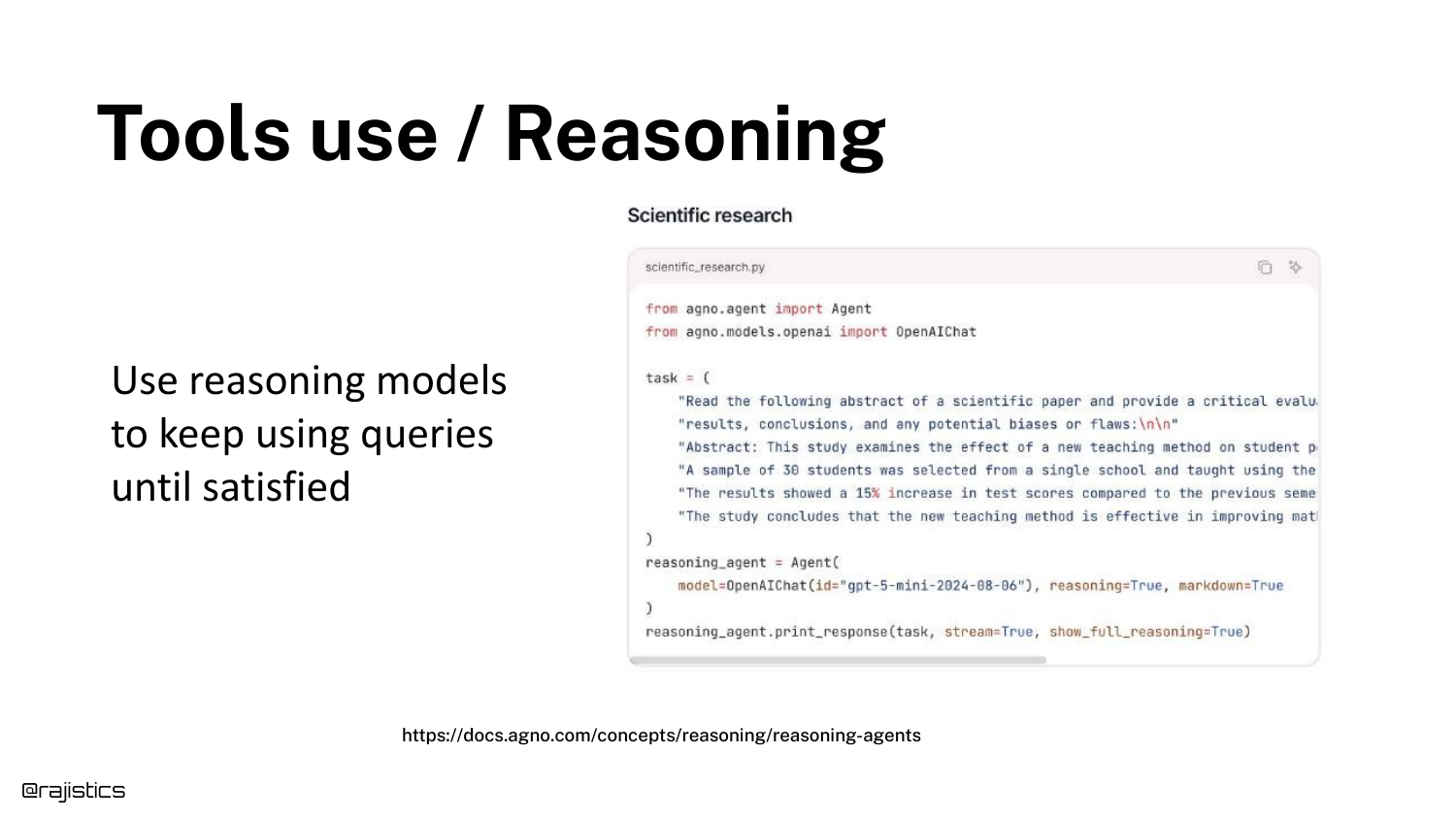
Reasoning models (like o1 or DeepSeek R1) enable LLMs to use tools effectively. A code snippet shows an agent loop: query -> generate -> “Did it answer the question?”
If the answer is no, the model can “rewrite the query… try to find that missing information, feed that back into the loop.” This self-correction is the core of Agentic RAG.
48. Agentic RAG (Workflow)
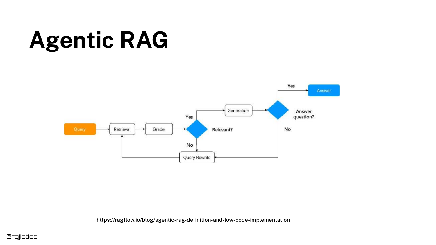
A flowchart details the Agentic RAG lifecycle. The model thinks through steps: “Oh, this is the query I need to make… based on those results… maybe we should do it a different way.”
This workflow allows the system to synthesize answers from multiple sources or clarify ambiguous queries automatically.
49. Tools use / Reasoning (Detailed Example)
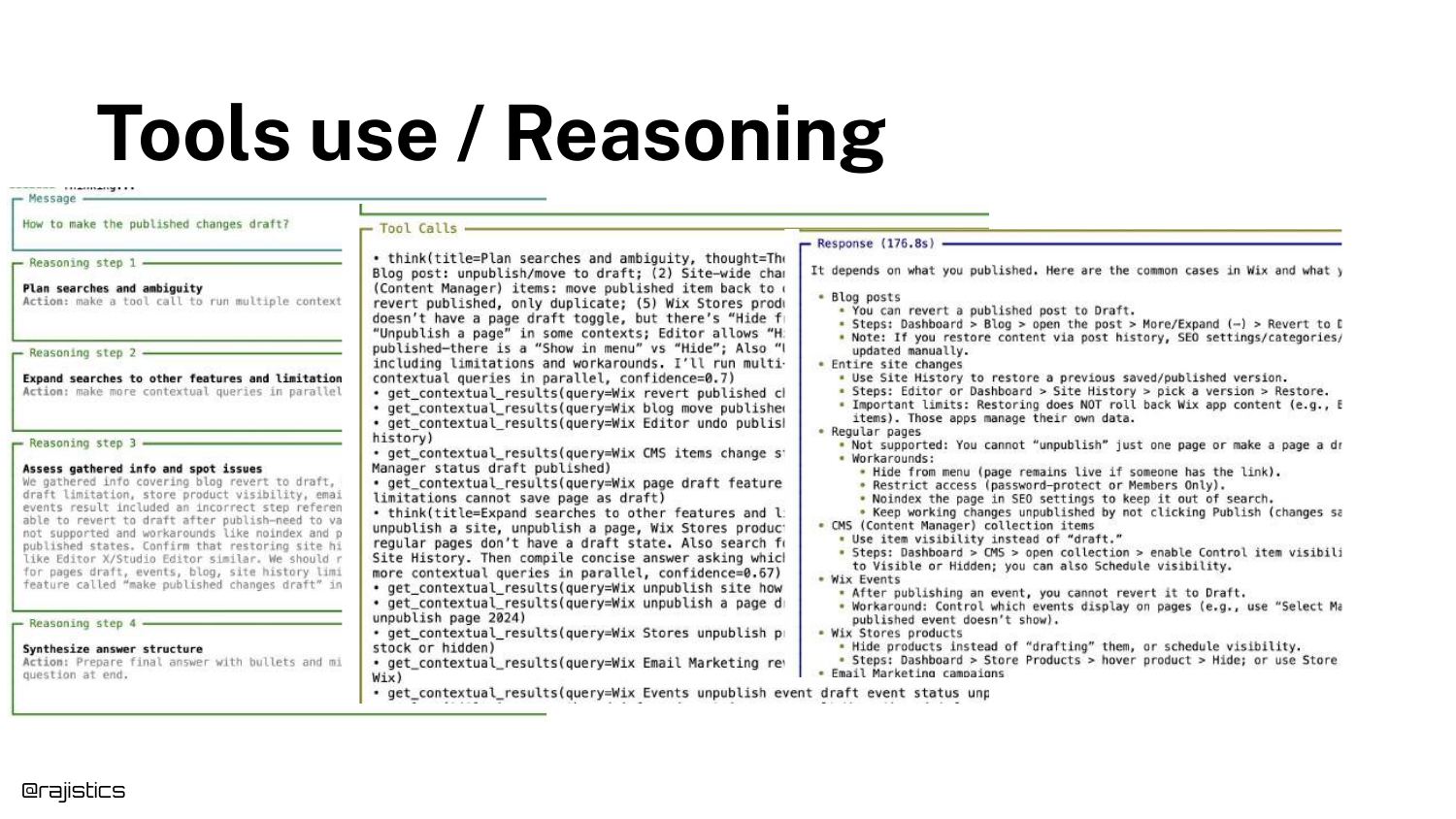
A specific example of a complex query is shown. The agent breaks the problem down, calls tools, and iterates.
This demonstrates that the “Thinking” time is where the value is generated, allowing for a depth of research that a single retrieval pass cannot match.
50. Open Deep Research
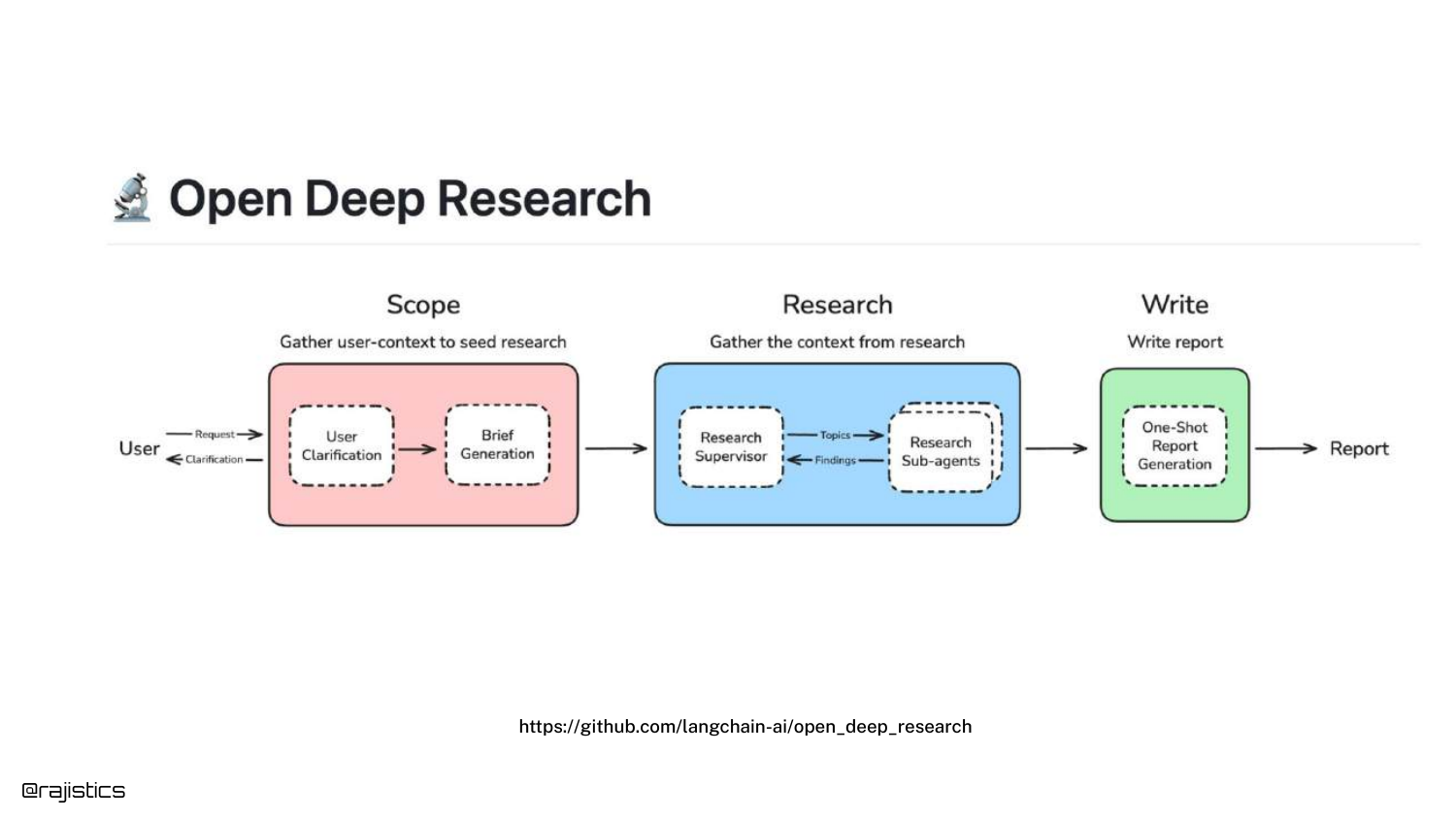
Shah references “Open Deep Research” by LangChain, an open-source framework where sub-agents go out, perform research, and report back.
This is a specific category of Agentic RAG focused on generating comprehensive reports rather than quick answers.
51. DeepResearch Bench
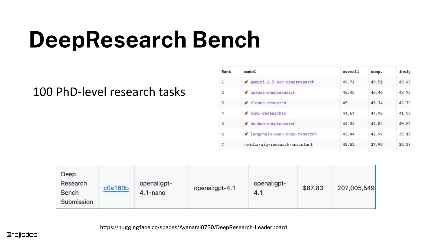
A leaderboard for DeepResearch Bench is shown, testing models on “100 PhD level research tasks.”
The speaker warns that this approach “can get very expensive.” Solving a single complex query might cost significant money due to the number of tokens and iterative steps required.
52. Westlaw AI Deep Research
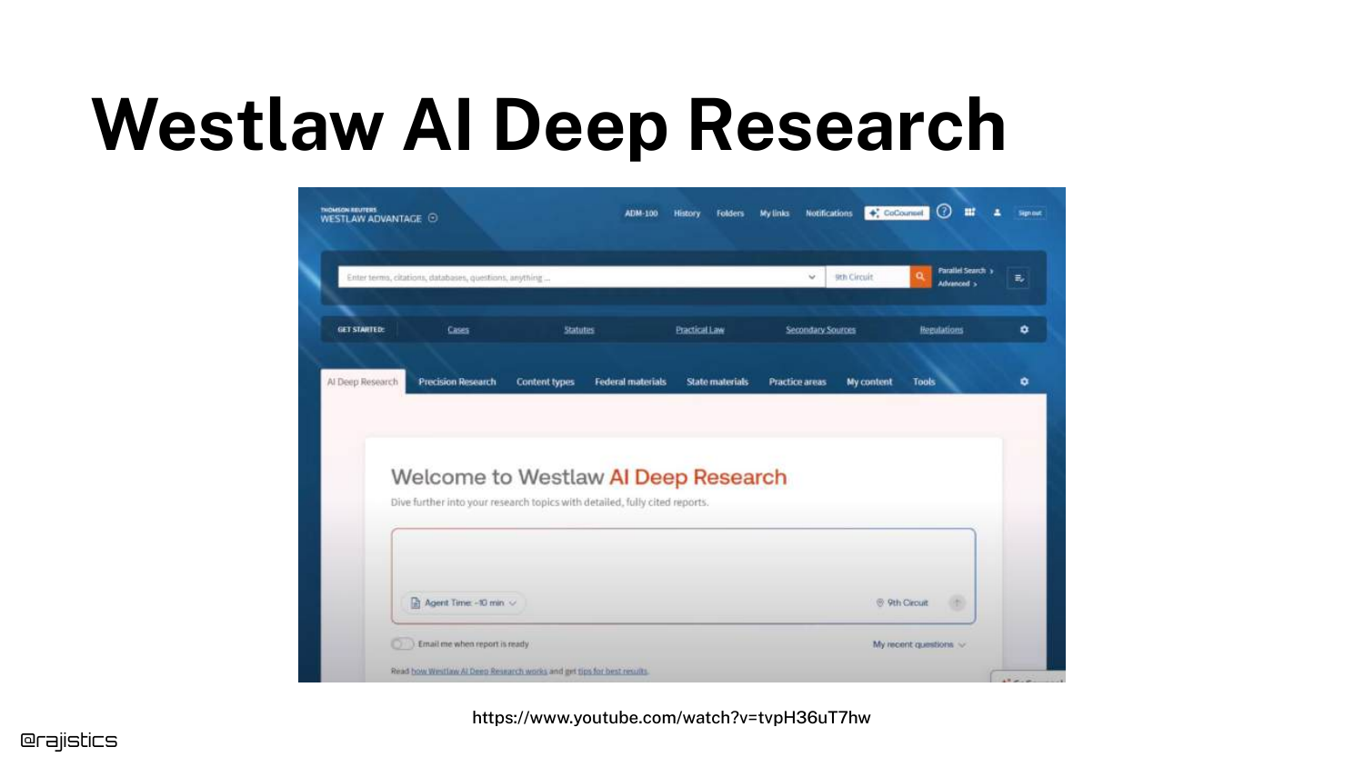
A real-world application is highlighted: Westlaw AI. In the legal field, thoroughness is worth the latency and cost.
This proves that Agentic RAG isn’t just a toy; it is being commercialized in high-value verticals where accuracy is paramount.
53. Agentic RAG (Self-RAG)
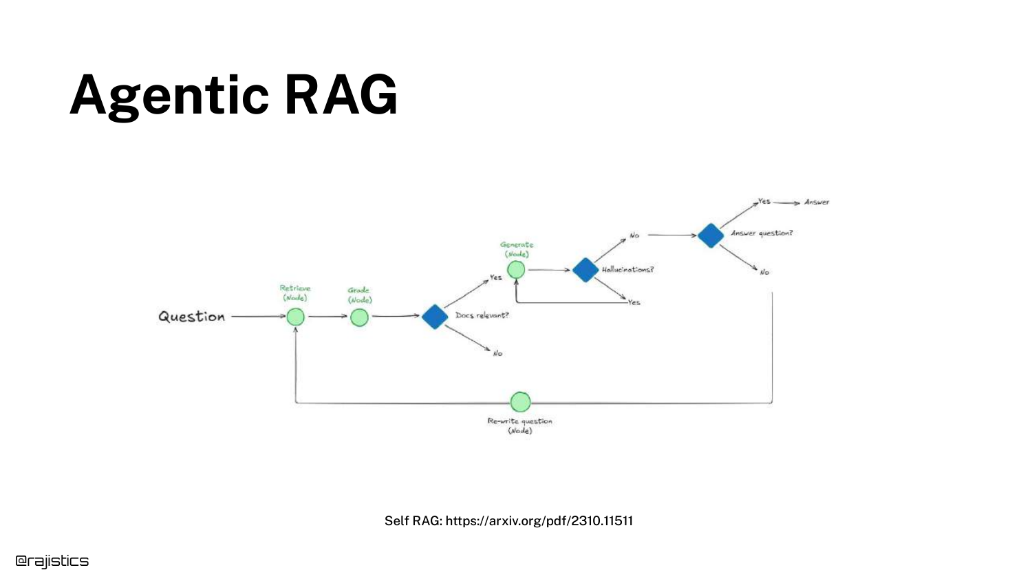
The concept of Self-RAG is introduced, emphasizing the “Reflection” step. The model critiques its own retrieved documents and generation quality.
Shah notes that this isn’t brand new, but has become practical due to better reasoning models.
54. Agentic RAG (LangChain Reddit)
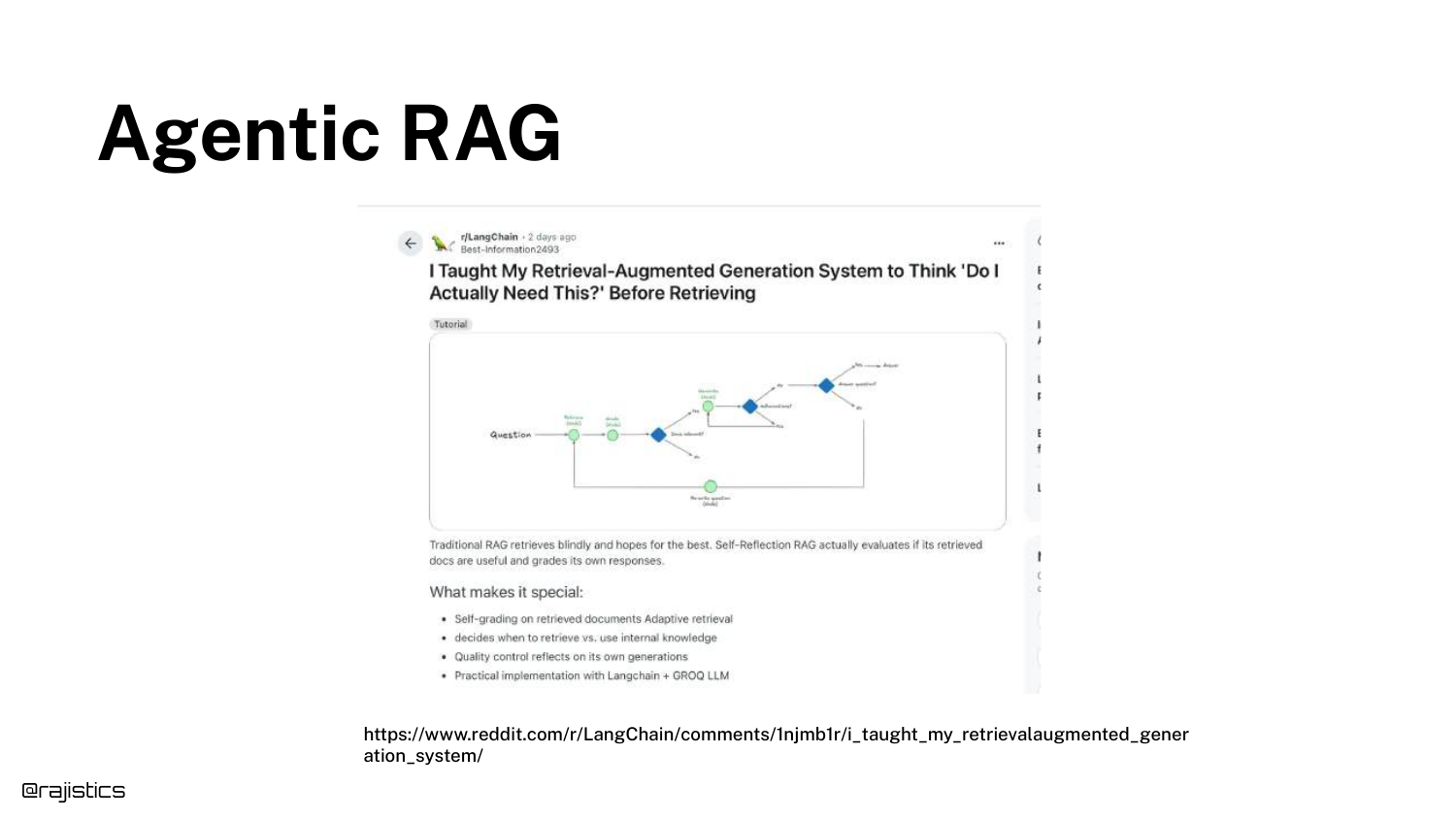
A Reddit post is shown where a developer discusses building a self-reflection RAG system. This highlights the community’s active experimentation with these loops.
55. Agentic RAG (Efficiency Concerns)
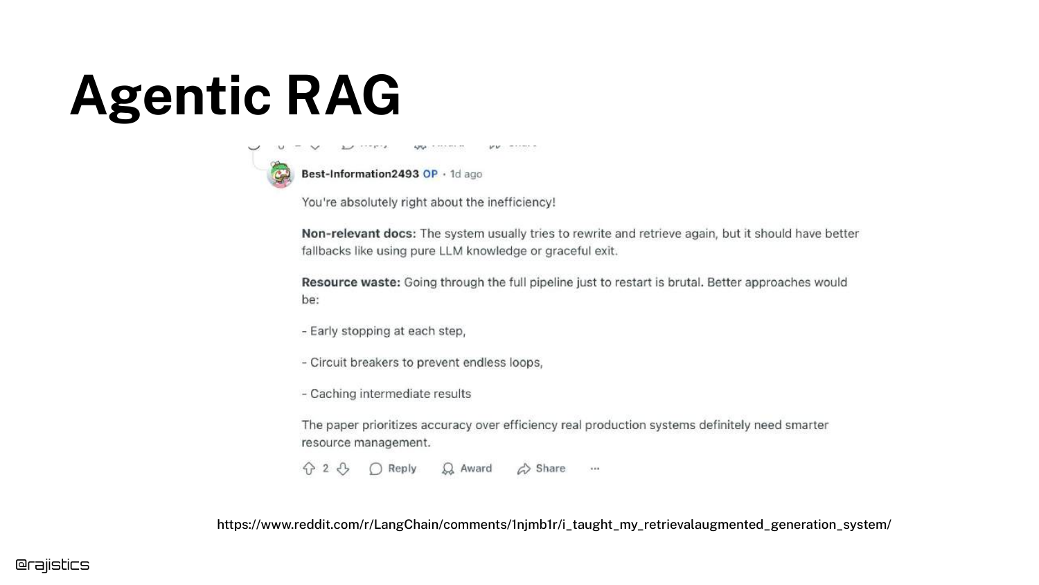
The discussion turns to the “Rub”: Inefficiency. Agentic loops can be slow and wasteful, re-retrieving data unnecessarily.
This sets up the trade-off conversation again: Is the extra time and compute worth the accuracy gain?
56. Research: BRIGHT
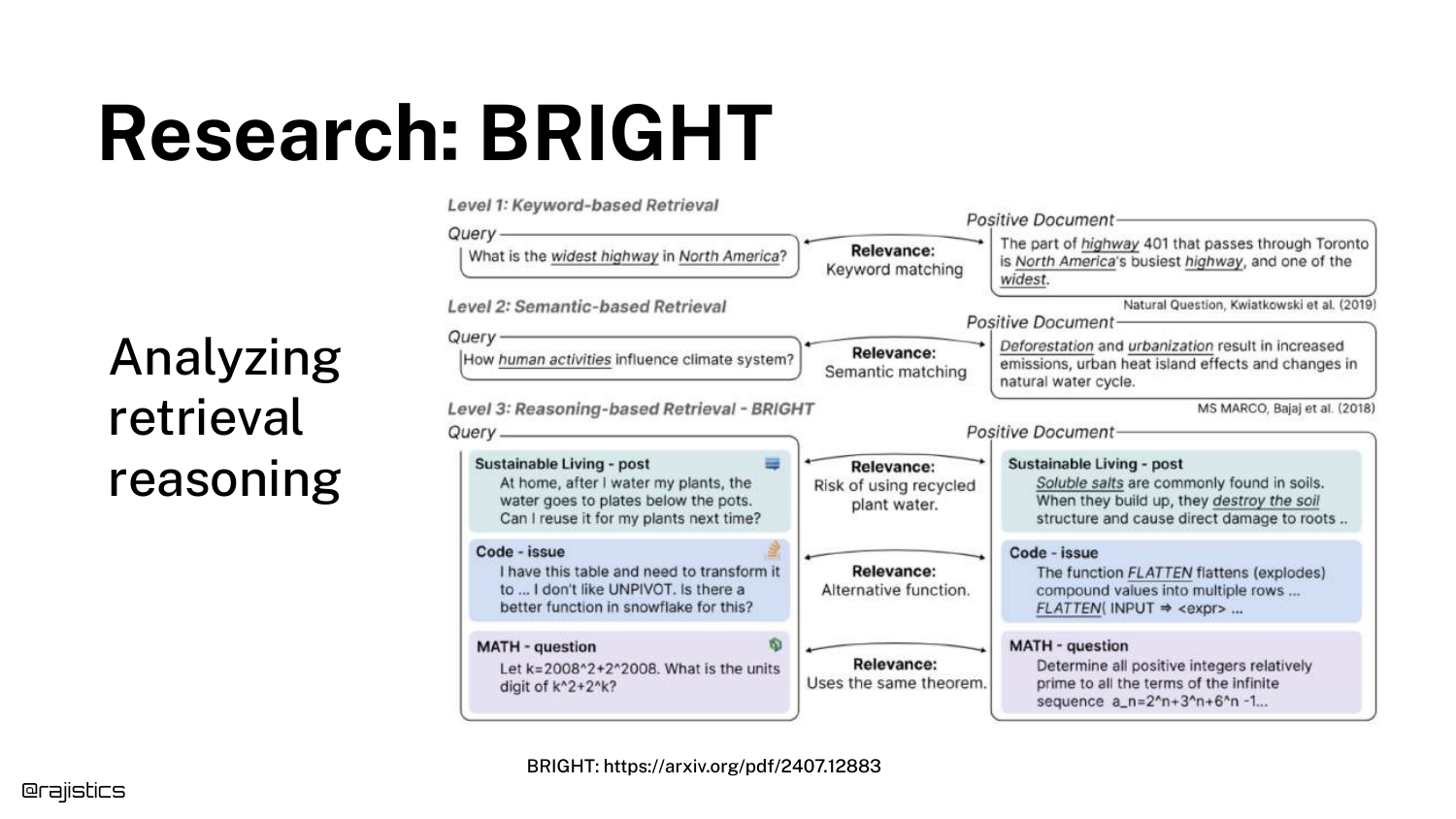
Note: The speaker introduces the BRIGHT benchmark around 32:11, slightly out of slide order in the transcript flow, but connects it here.
BRIGHT is a benchmark specifically designed for Retrieval Reasoning. Unlike standard benchmarks that test keyword matching, BRIGHT tests questions that require thinking, logic, and multi-step deduction to find the correct document.
57. BRIGHT #1: DIVER
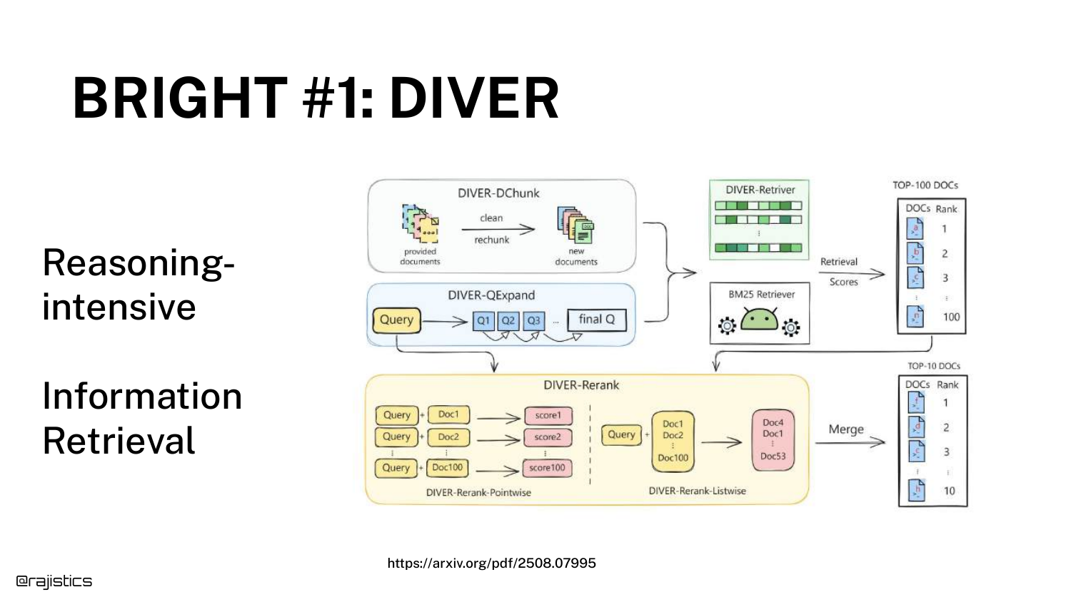
The top-performing system on BRIGHT is DIVER. The diagram shows it uses the exact components discussed earlier: Chunking, Retrieving, and Reranking, but wrapped in an iterative loop.
Shah points out, “It probably doesn’t look that crazy to you if you’re used to RAG.” The innovation is in the process, not necessarily a magical new model architecture.
58. BRIGHT #1: DIVER (LLM Instructions)
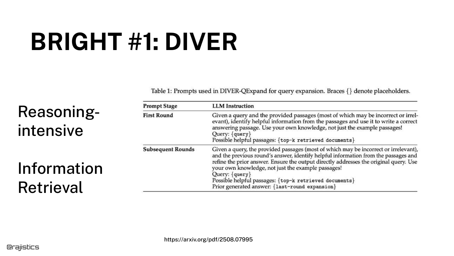
The specific prompts used in DIVER are shown. The system asks the LLM: “Given a query… what do you think would be possibly helpful to do?”
This Query Expansion allows the system to generate new search terms that the user didn’t think of, bridging the semantic gap through reasoning.
59. Agentic RAG on WixQA
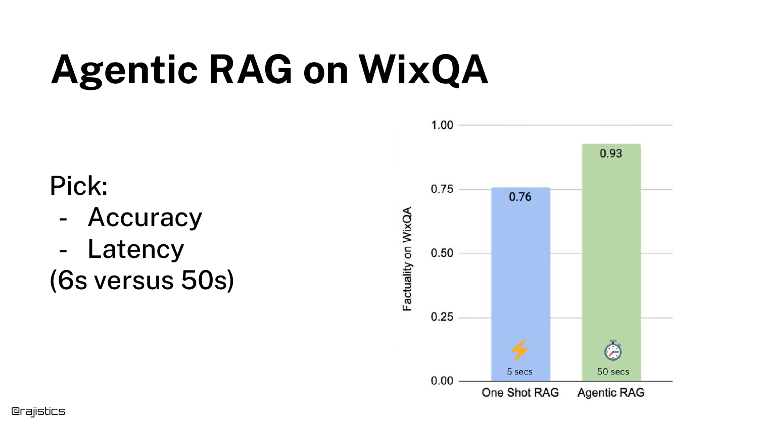
Shah shares his own experiment results on the WixQA dataset (technical support). * One Shot RAG: 5 seconds latency, 76% Factuality. * Agentic RAG: Slower latency, 93% Factuality.
This massive jump in accuracy (0.76 to 0.93) is the key takeaway. “That has a ton of implications.” It suggests that the limitation of RAG often isn’t the data, but the lack of reasoning applied to the retrieval process.
60. Rethink your Assumptions
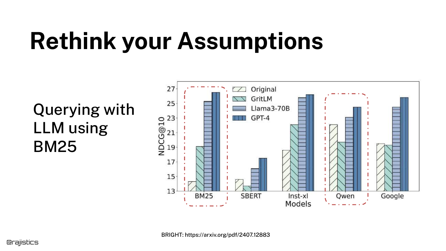
This is the climax of the technical argument. A graph from the BRIGHT paper shows that BM25 (lexical search) combined with an Agentic loop (GPT-4) outperforms advanced embedding models (Qwen).
“This is crazy,” Shah exclaims. Because the LLM can rewrite queries into many variations, it mitigates BM25’s weakness (synonyms). This implies you might not need complex vector databases if you have a smart agent.
61. Agentic RAG with BM25
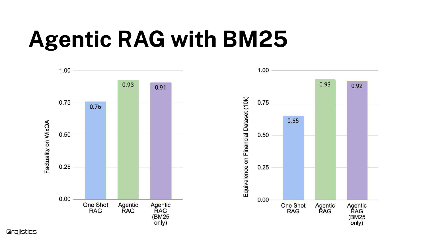
Shah validates the paper’s finding with his own internal data (Financial 10Ks). Agentic RAG with BM25 performed nearly as well as Agentic RAG with Embeddings.
He suggests a radical possibility: “I could throw all that away [vector DBs]… just stick this in a text-only database and use BM25.”
62. Agentic RAG for Code Search
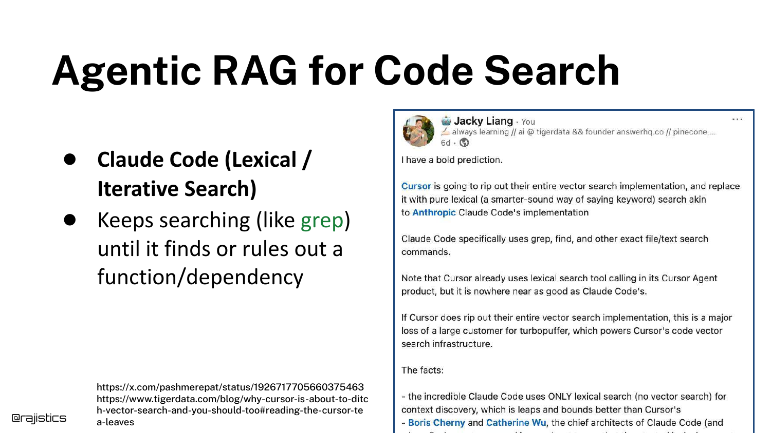
He connects this finding to Claude Code, which uses a lexical approach (like grep) rather than vectors for code search.
Since code doesn’t have the same semantic ambiguity as natural language, and agents can iterate rapidly, lexical search is proving to be superior for coding assistants.
63. Combine Retrieval Approaches
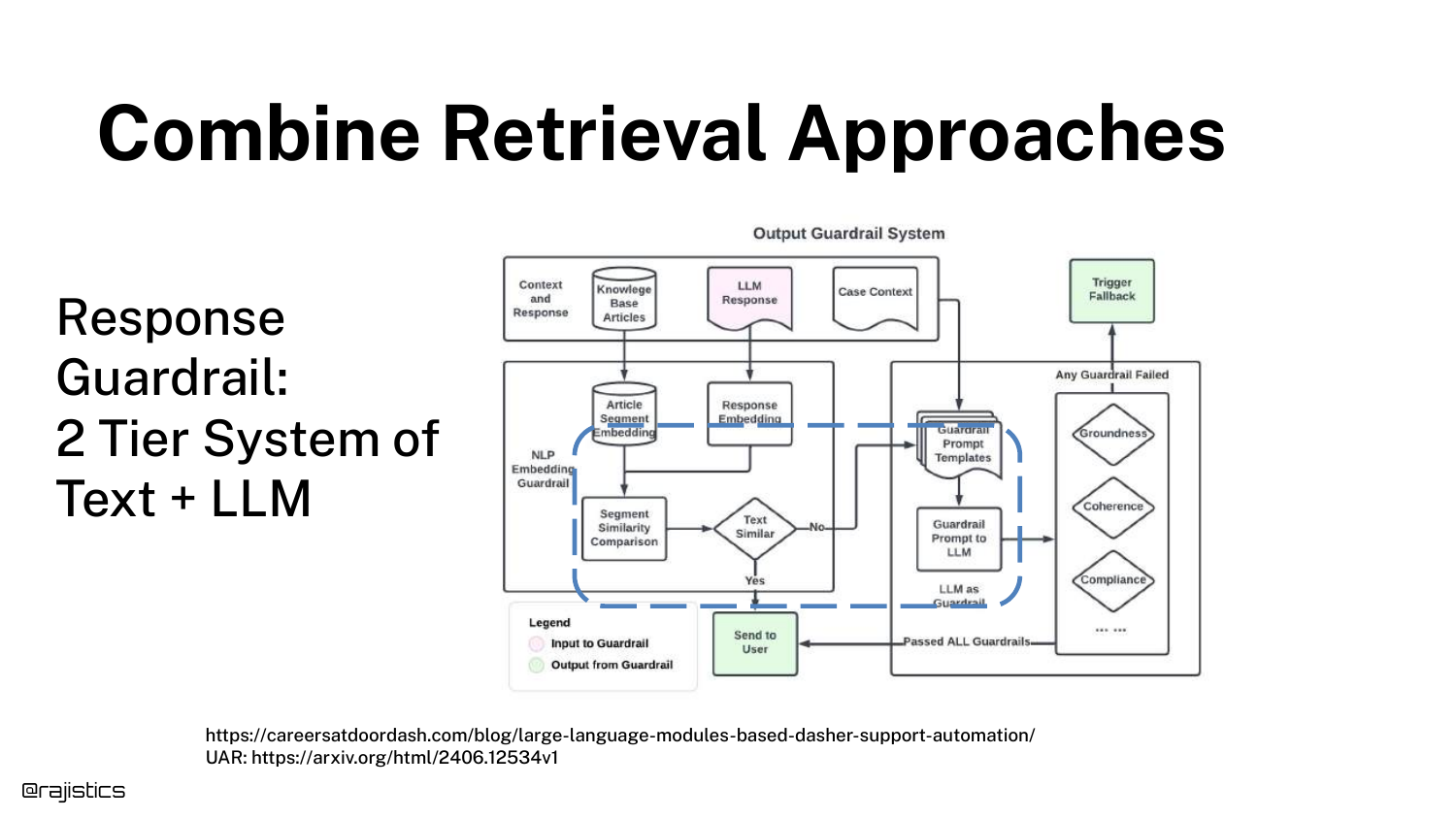
A DoorDash case study illustrates a two-tier guardrail system. They use simple text similarity first (fast/cheap). If that fails or is uncertain, they kick it to an LLM (slow/expensive).
This “Tiered” approach optimizes the trade-off between cost and accuracy in production.
64. Hands on: Agentic RAG (Smolagents)
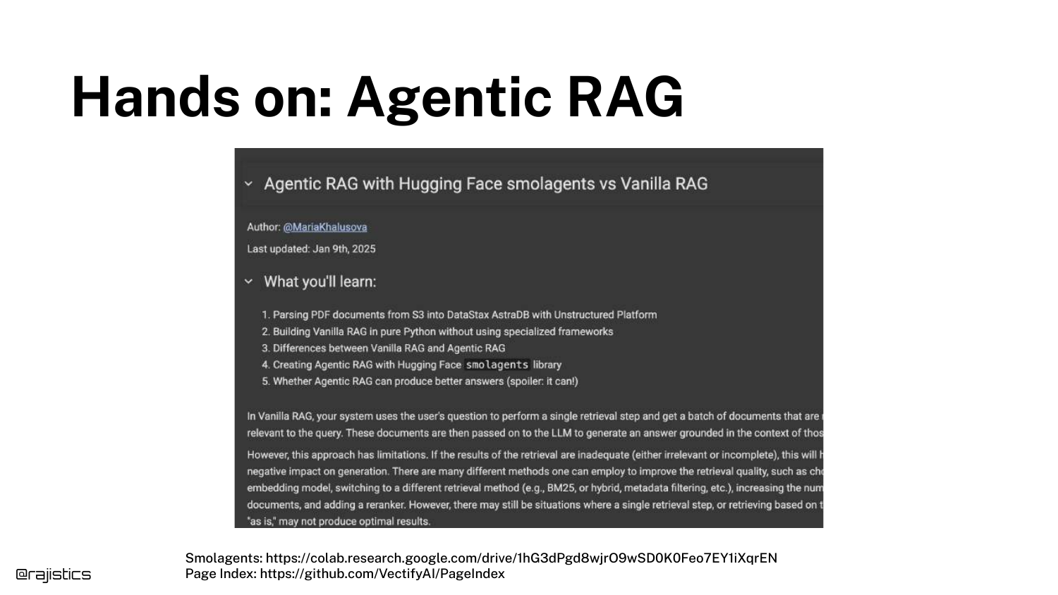
The speaker points to Smolagents, a Hugging Face library, as a way to get hands-on with these concepts. A Colab notebook is provided for the audience to build their own agentic retrieval loops.
65. Solutions for a RAG Solution
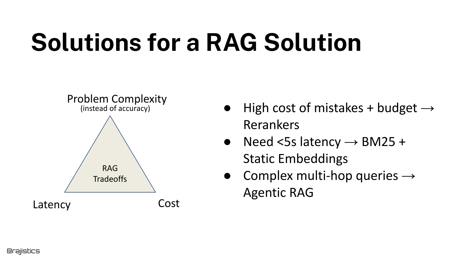
Shah updates the “Problem Complexity” framework from the beginning of the talk with specific recommendations: * Low Latency (<5s): Use BM25 or Static Embeddings. * High Cost of Mistake: Add a Reranker. * Complex Multi-hop: Use Agentic RAG.
66. Retriever Checklist
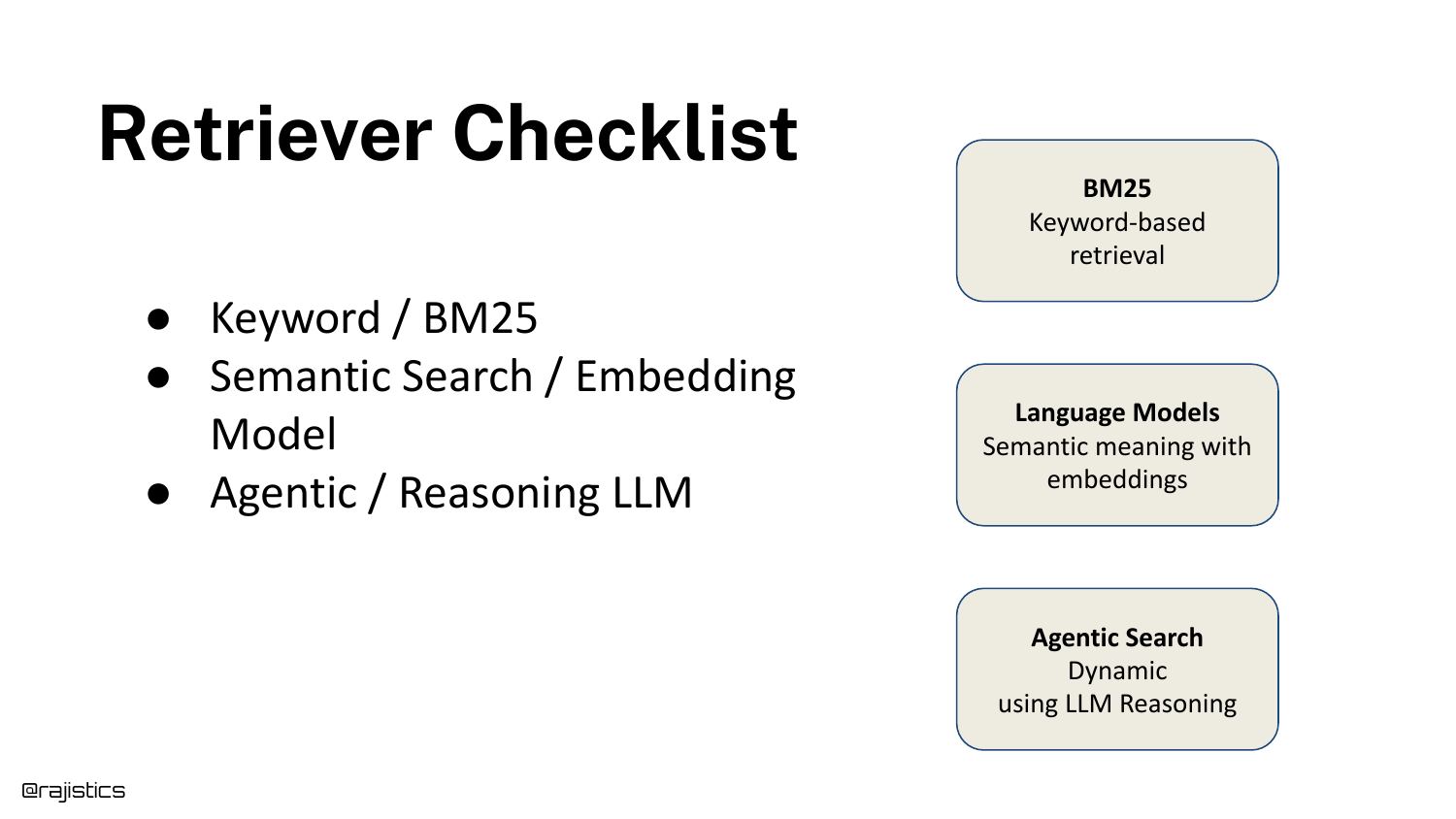
A final checklist summarizes the retrieval hierarchy: 1. Keyword/BM25 (The baseline). 2. Semantic Search (The standard). 3. Agentic/Reasoning (The problem solver).
This provides the audience with a mental menu to choose from based on their specific constraints.
67. RAG as a system (Retrieval with Instruction Following Reranker)
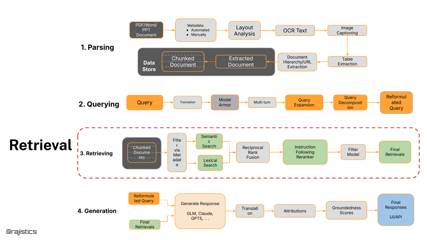
The system diagram is shown one last time, updated to include the Instruction Following Reranker in the retrieval box, solidifying the modern RAG architecture.
68. RAG - Generation
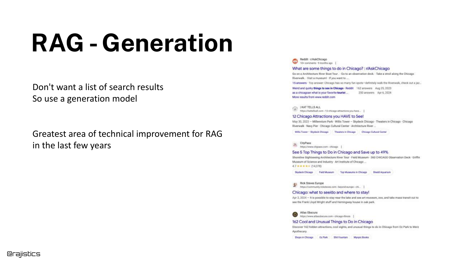
Note: The speaker concludes the talk at 42:10, stating “I’m going to end it here.” Slides 68-70 regarding the Generation stage were included in the deck but skipped in the video recording due to time constraints.
This slide would have covered the final stage of RAG: generating the answer. The focus here is typically on reducing hallucinations and ensuring the tone matches the user’s needs.
69. RAG - Generation (Model Selection)
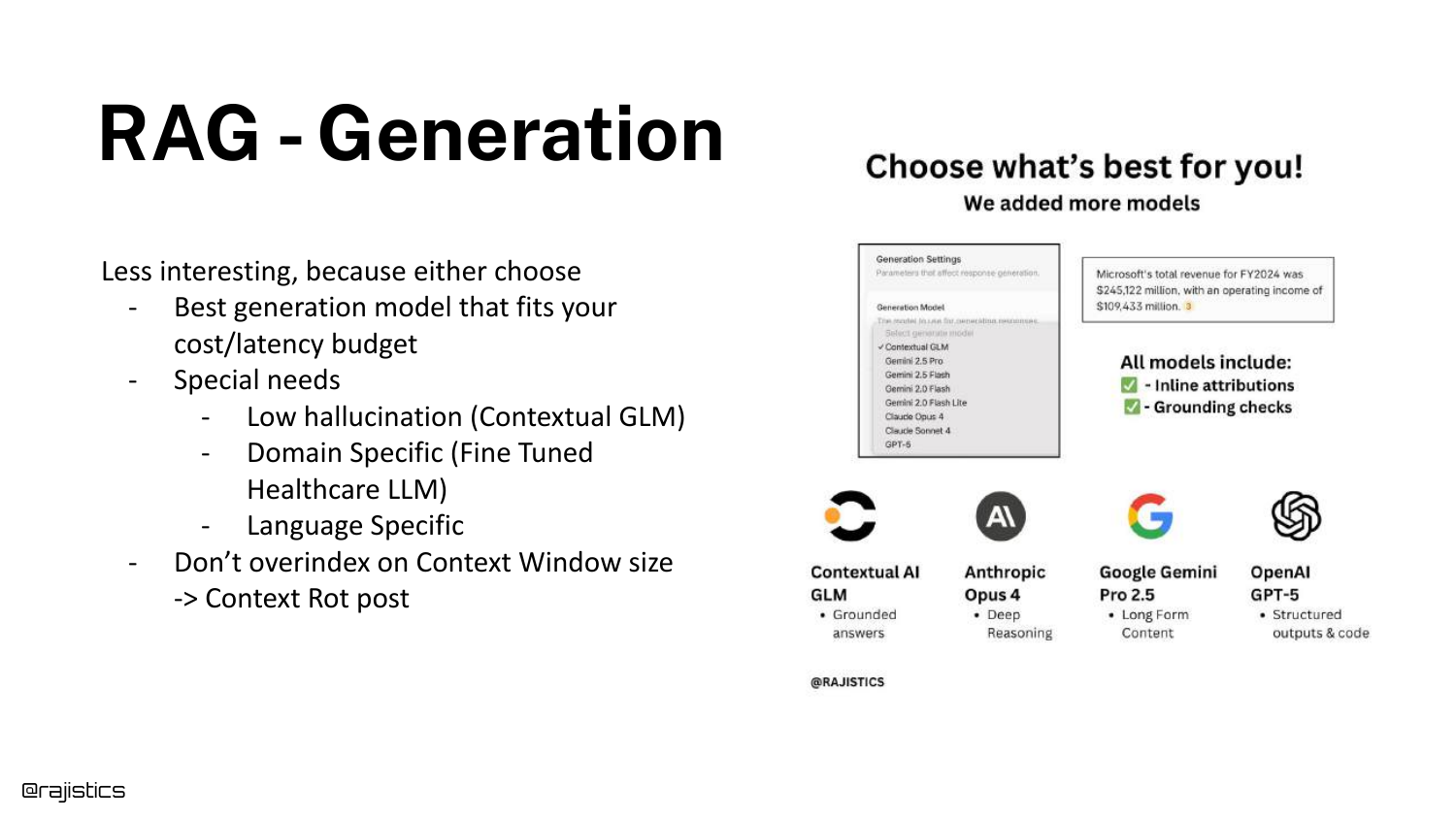
Skipped in video. This slide illustrates the choice of LLM for generation (e.g., GPT-4 vs Llama 3 vs Claude). The choice depends on the “Cost/Latency budget” and specific domain requirements.
70. Chunking approaches
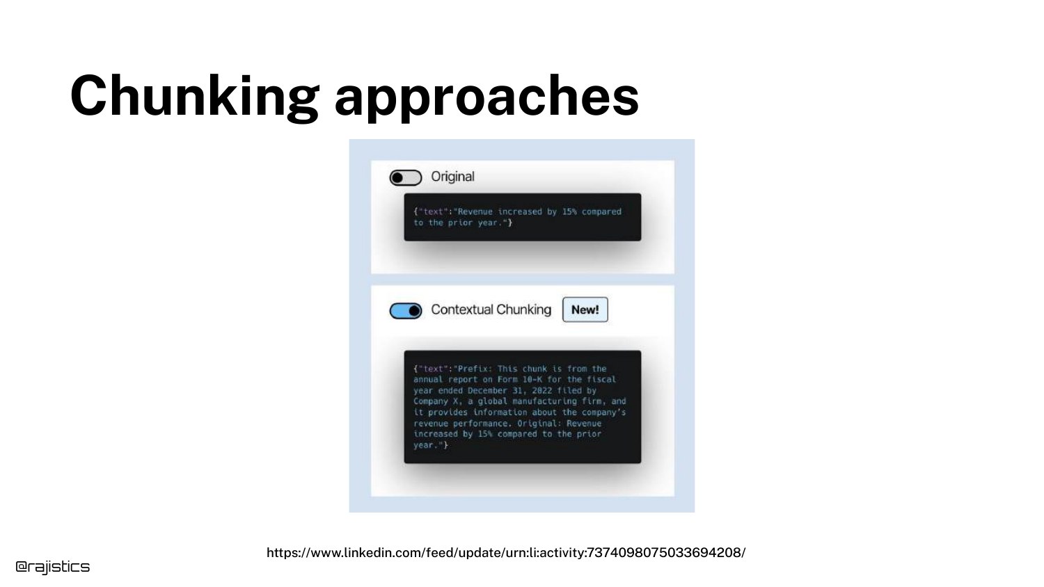
Skipped in video. This slide compares Original Chunking (cutting text at fixed intervals) with Contextual Chunking (adding a summary prefix to every chunk). Contextual chunking significantly improves retrieval because every chunk carries the context of the parent document.
71. Title Slide (Duplicate)
The presentation concludes with the title slide. Rajiv Shah thanks the audience, encouraging them to think about trade-offs rather than just chasing the latest models. “Hopefully I’ve given you a sense of thinking about these trade-offs… thank you all.”
This annotated presentation was generated from the talk using AI-assisted tools. Each slide includes timestamps and detailed explanations.