Video
Watch the full video
Annotated Presentation
Below is an annotated version of the presentation, with timestamped links to the relevant parts of the video for each slide.
Here is the annotated presentation for “Evaluating LLMs” by Rajiv Shah.
1. Title Slide: Evaluating LLMs

The presentation begins with the title slide, introducing the speaker, Rajiv Shah, and the topic of Evaluating Large Language Models (LLMs). The slide includes a link to a GitHub repository (LLM-Evaluation), which serves as a companion resource containing notebooks and code examples referenced throughout the talk.
Rajiv sets the stage by explaining his motivation: he sees many enterprises treating Generative AI as “science experiments” that fail to reach production. He argues that a major reason for this failure is a lack of proper evaluation strategies.
The goal of this talk is to move beyond experimentation and discuss how to rigorously evaluate models to get them into production and keep them there, covering technical, business, and operational perspectives.
2. No Impact!
This slide humorously illustrates the current state of many LLM projects. It depicts a chaotic lab scene and a cartoon character in a strange vehicle, captioned “No impact!” This visualizes the frustration of data scientists building cool things that never deliver real-world value.
Rajiv uses this to highlight the “science experiment” nature of current GenAI work. Without proper evaluation, teams cannot prove the reliability or value of their models, preventing deployment.
The slide emphasizes the necessity of shifting from “playing around” with models to applying rigorous engineering discipline, starting with evaluation.
3. Three Pillars of Evaluation
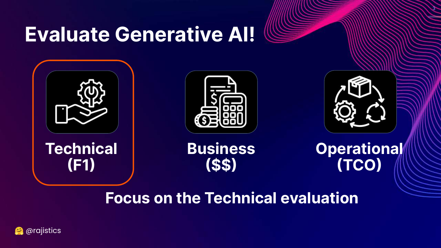
This slide breaks down Generative AI evaluation into three critical dimensions: Technical (F1), Business ($$), and Operational (TCO). While the talk focuses heavily on technical metrics, Rajiv stresses that the other two are equally vital for production success.
The Business dimension asks about the return on investment and the cost of errors, while the Operational dimension considers the Total Cost of Ownership (TCO), latency, and maintenance.
Understanding all three pillars is what distinguishes a successful production deployment from a mere prototype.
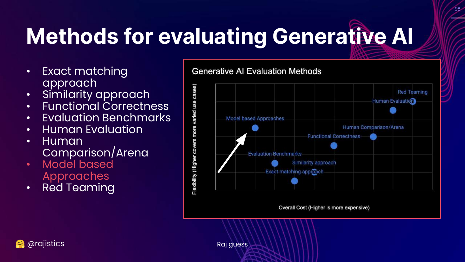
4. Generative AI Evaluation Methods

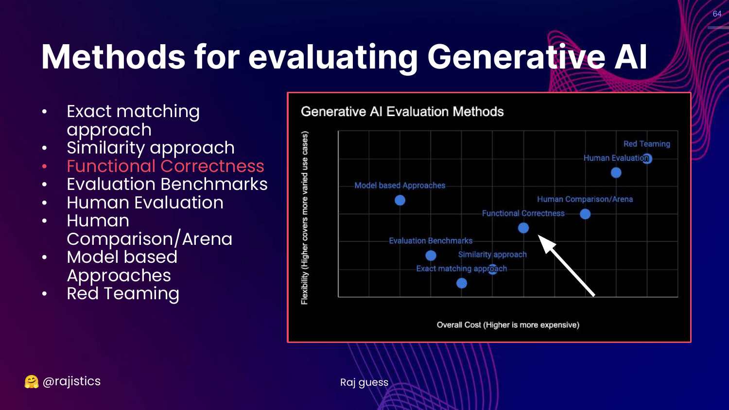
This chart is the central framework of the presentation. It categorizes technical evaluation methods based on Cost (y-axis) and Flexibility (x-axis). The methods range from rigid, low-cost approaches like Exact Matching to flexible, high-cost approaches like Red Teaming.
The slide lists specific methodologies: Exact matching, Similarity (BLEU/ROUGE), Functional correctness (Unit tests), Benchmarks (MMLU), Human evaluation, Model-based approaches (LLM-as-a-Judge), and Red teaming.
Rajiv notes that these categories overlap and are not mutually exclusive. This visual guide helps practitioners choose the right tool for their specific stage of development and resource constraints.
5. Application to RAG
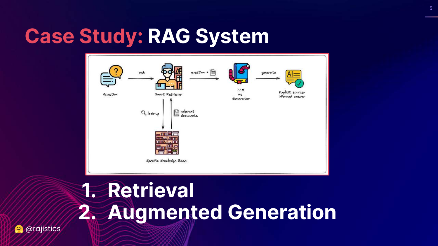
This slide previews the case study at the end of the talk: Retrieval Augmented Generation (RAG). It shows a diagram splitting the RAG process into two distinct components: Retrieval (finding the data) and Augmented Generation (synthesizing the answer).
Rajiv introduces this here to promise a practical application of the concepts. He explains that after covering the evaluation methods, he will demonstrate how to apply them specifically to a RAG system.
This foreshadows the importance of component-wise evaluation—evaluating the retriever and the generator separately rather than just the system as a whole.
6. Evaluating LLMs (Title Repeat)

This slide serves as a transition point, reiterating the talk’s title and contact information. It signals the end of the introduction and the beginning of the deep dive into the current state of LLMs.
Rajiv notes that this will be a long, detailed talk, encouraging viewers to use the video timeline to skip around. He sets expectations for the pace and depth of the technical content to follow.
7. Many Ways to Use LLMs
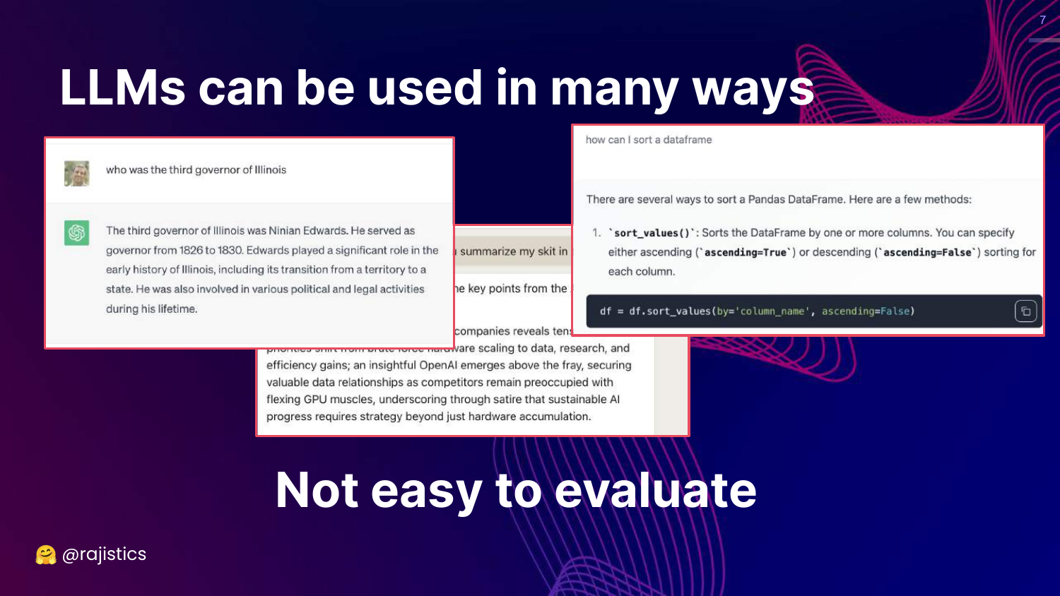
This slide illustrates the versatility of LLMs, showing examples of Question Answering and Code Generation. It highlights that LLMs are not limited to a single task like classification; they can summarize, chat, write code, and reason.
Rajiv explains that this versatility makes evaluation difficult. Unlike traditional ML where a simple confusion matrix might suffice, LLMs produce varied, open-ended outputs that require more complex assessment strategies.
The slide sets up the problem statement: because LLMs can do so much, we need a diverse set of evaluation tools to measure their performance across different modalities.
8. Open Source LLM Leaderboard
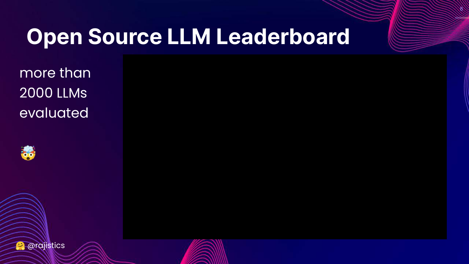
This slide shows a screenshot of the Hugging Face Open LLM Leaderboard. It notes that over 2,000 LLMs have been evaluated, visualizing the sheer volume of models available to practitioners.
Rajiv describes the experience of looking for a model as “overwhelming.” With new models releasing weekly, relying solely on public leaderboards to pick a model is daunting and potentially misleading.
This introduces the concept of “Leaderboard Fatigue” and questions whether these general-purpose rankings are useful for specific enterprise use cases.
9. HELM Framework
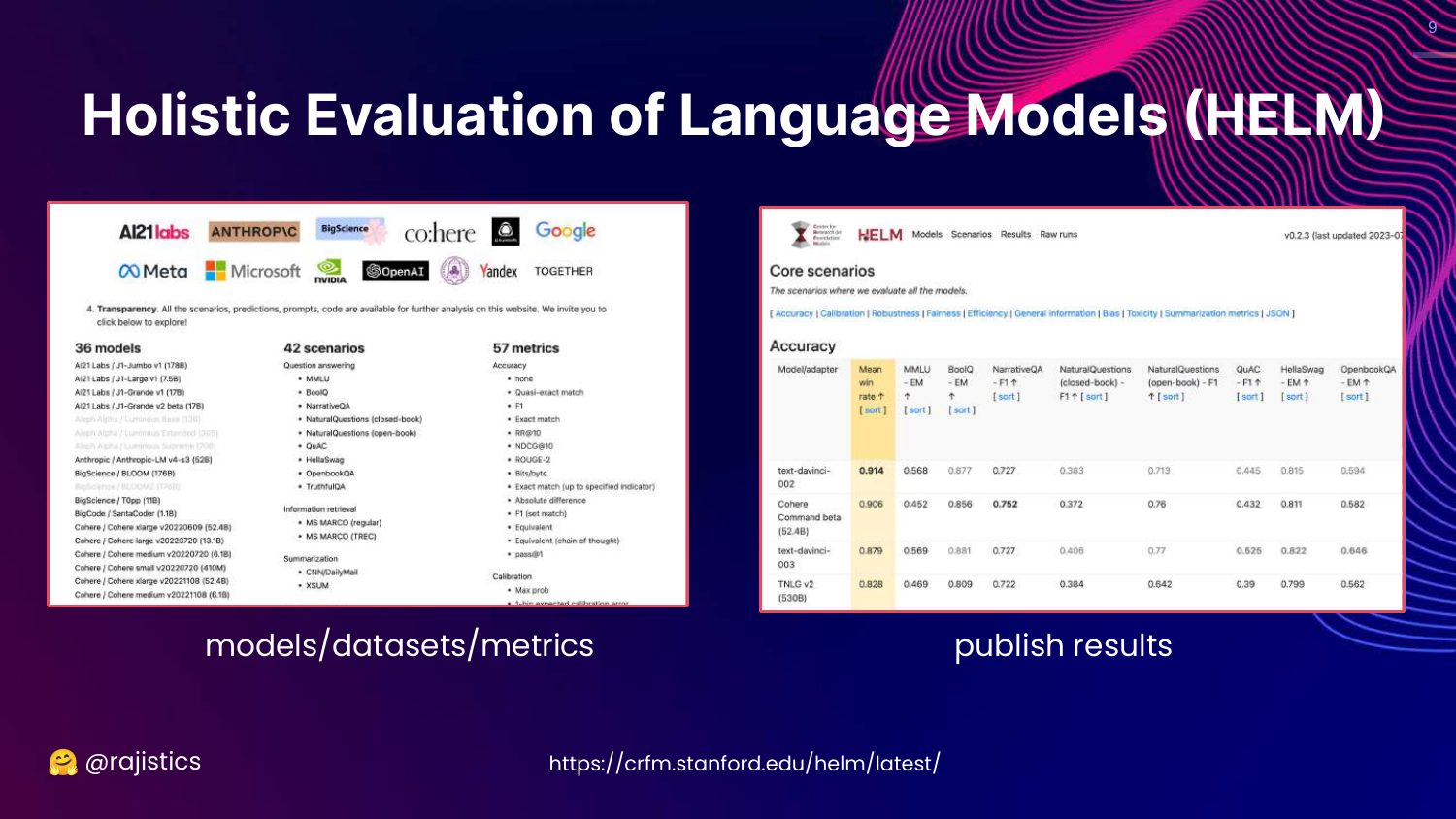
This slide introduces HELM (Holistic Evaluation of Language Models) from Stanford. It displays the framework’s structure, which evaluates models across various scenarios (datasets) and metrics (accuracy, bias, toxicity).
Rajiv presents HELM as the academic approach to the evaluation problem. It attempts to be comprehensive by measuring everything across many dimensions, offering a more rigorous alternative to simple leaderboards.
However, he points out that even this comprehensive approach has its downsides, primarily the sheer volume of data it produces.
10. Overwhelming Information
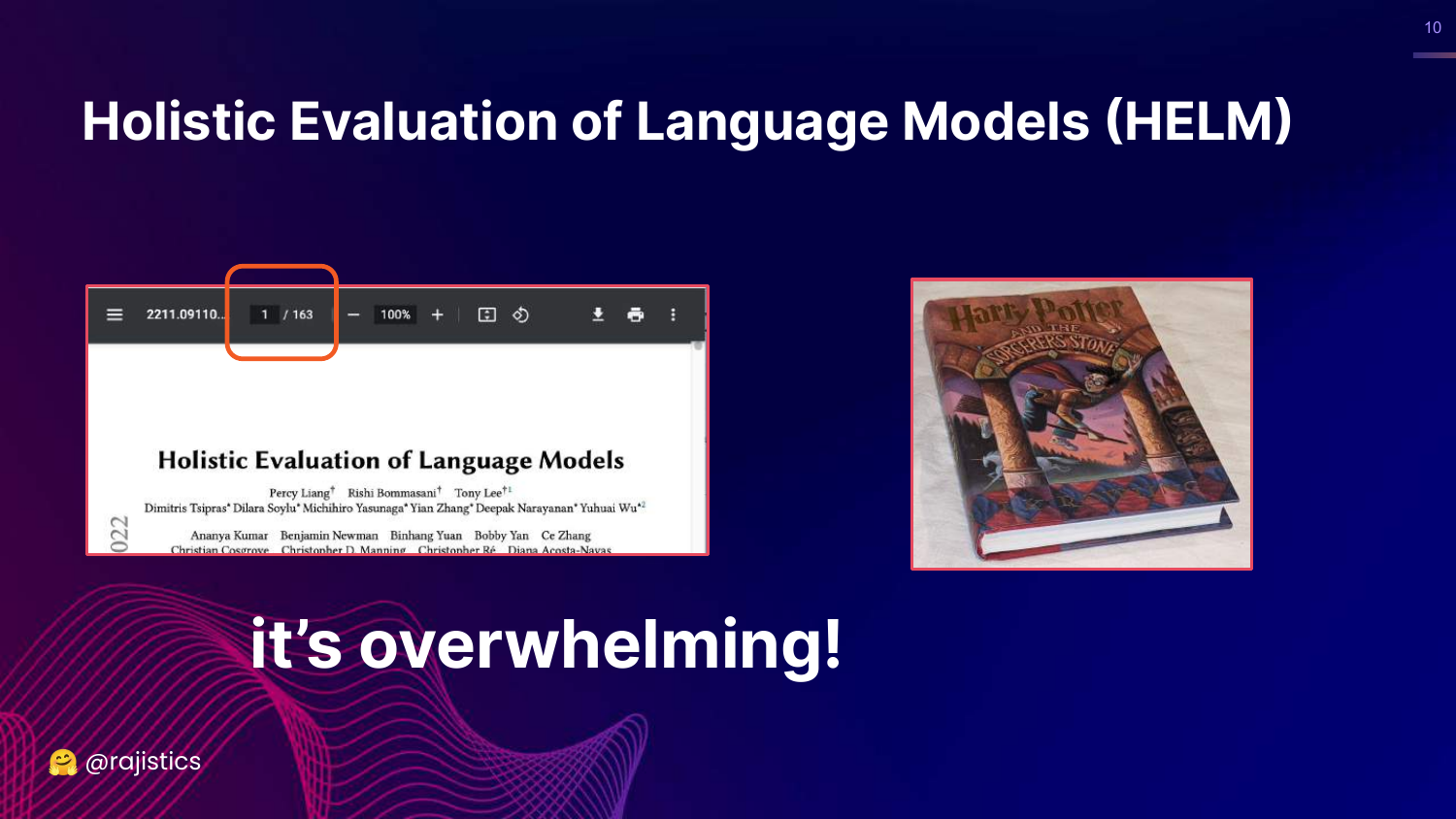
This slide displays a screenshot of the HELM research paper, emphasizing its length (163 pages). The caption “Overwhelming!” reflects the difficulty a data scientist faces when trying to digest this amount of information.
Rajiv humorously compares the paper’s size to a “Harry Potter book,” illustrating that while the academic rigor is high, the practical barrier to entry is also significant.
The key takeaway is that while comprehensive benchmarks exist, they are often too dense for quick, practical decision-making in an enterprise setting.
11. Feeling Overwhelmed

This visual slide features a person looking frustrated and burying their face in their hands. It represents the emotional state of a data scientist trying to navigate the complex, rapidly changing landscape of LLM evaluation.
Rajiv uses this to empathize with the audience. Between the thousands of models on Hugging Face and the hundreds of pages of academic papers, it is easy to feel lost.
This sets the stage for the need for simpler, more fundamental principles to guide evaluation.
12. Reliability of HELM
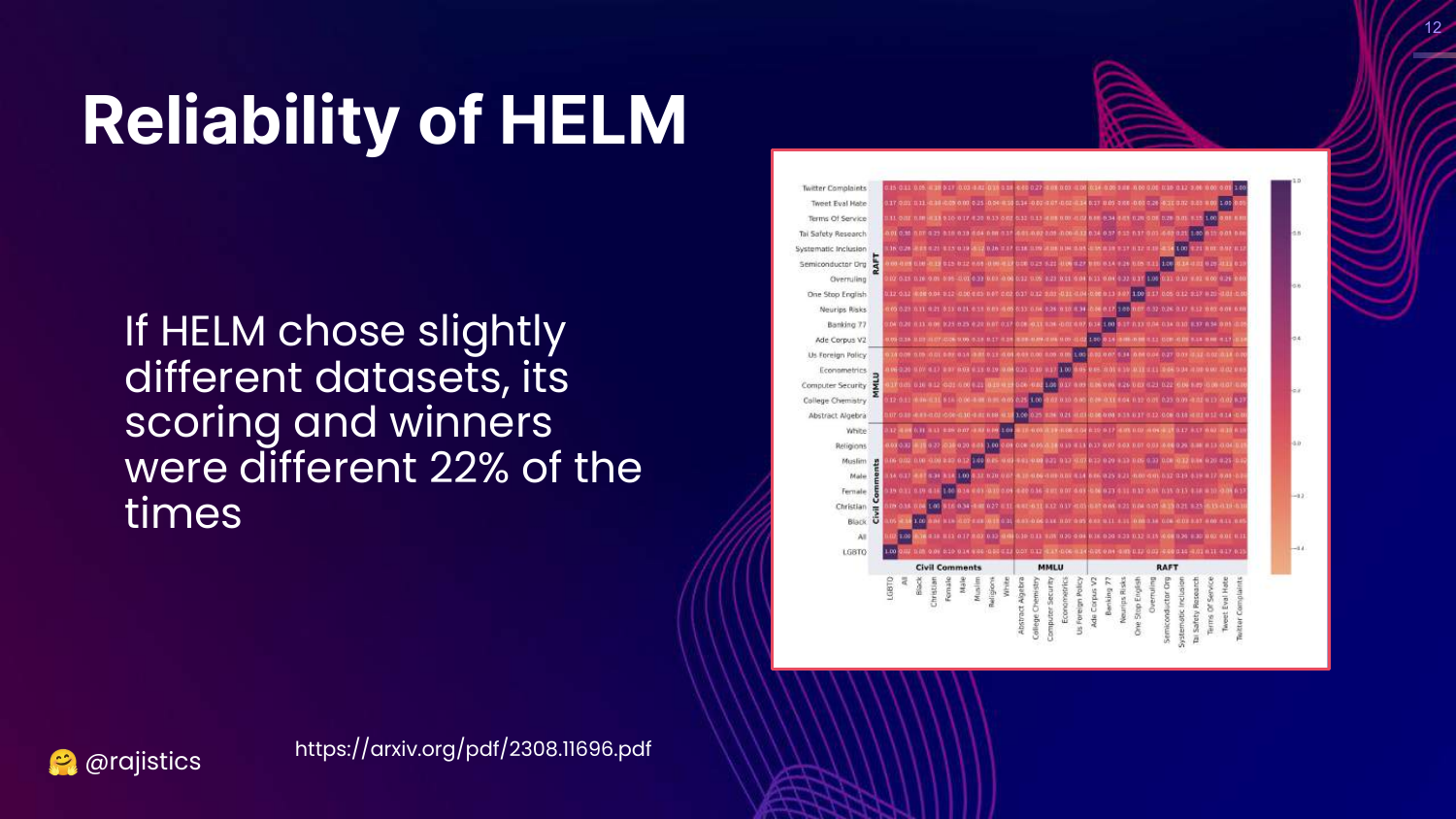
This slide questions the reliability of benchmarks like HELM. It presents data showing that minor changes in dataset selection can lead to different scoring and winners 22% of the time. A correlation matrix visualizes the relationships between different metrics.
Rajiv points out that benchmarks are fragile. If you change the specific datasets used to represent a “scenario,” the ranking of the models changes.
This implies that “winners” on leaderboards are often dependent on the specific composition of the benchmark rather than inherent superiority across all tasks.
13. Davinci-002 vs Davinci-003
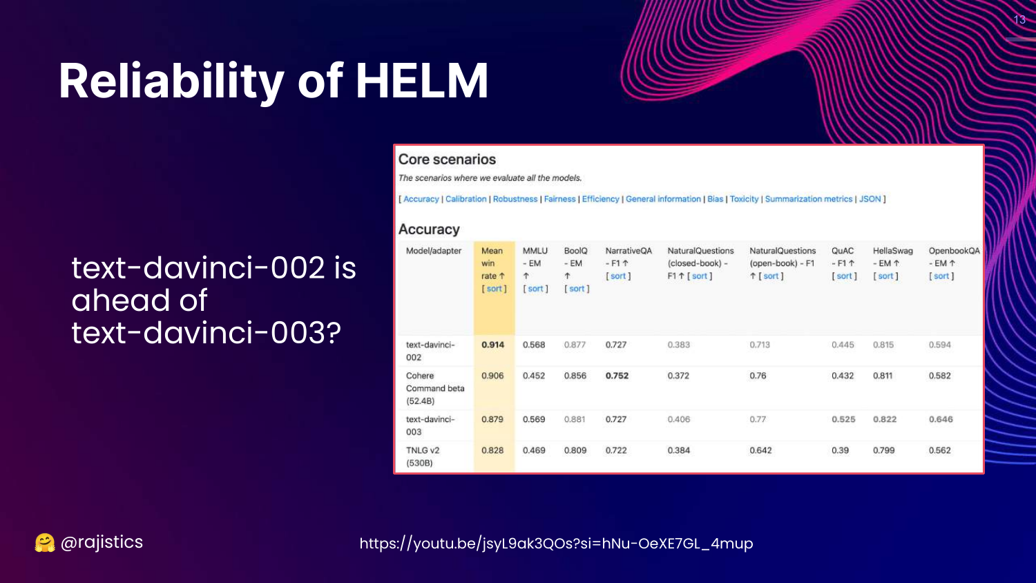
This slide highlights a specific anomaly in HELM results where an older model (text-davinci-002) appears to outperform a newer, better model (text-davinci-003) in accuracy.
Rajiv expresses skepticism, noting that OpenAI is unlikely to release a newer model that is objectively worse. This discrepancy suggests that the benchmark might not be capturing the improvements in the newer model, such as better instruction following or safety.
The slide serves as a warning: Do not blindly trust benchmark rankings, as they may not reflect the actual capabilities or “quality” of a model for your specific needs.
14. Leaderboard Reliability
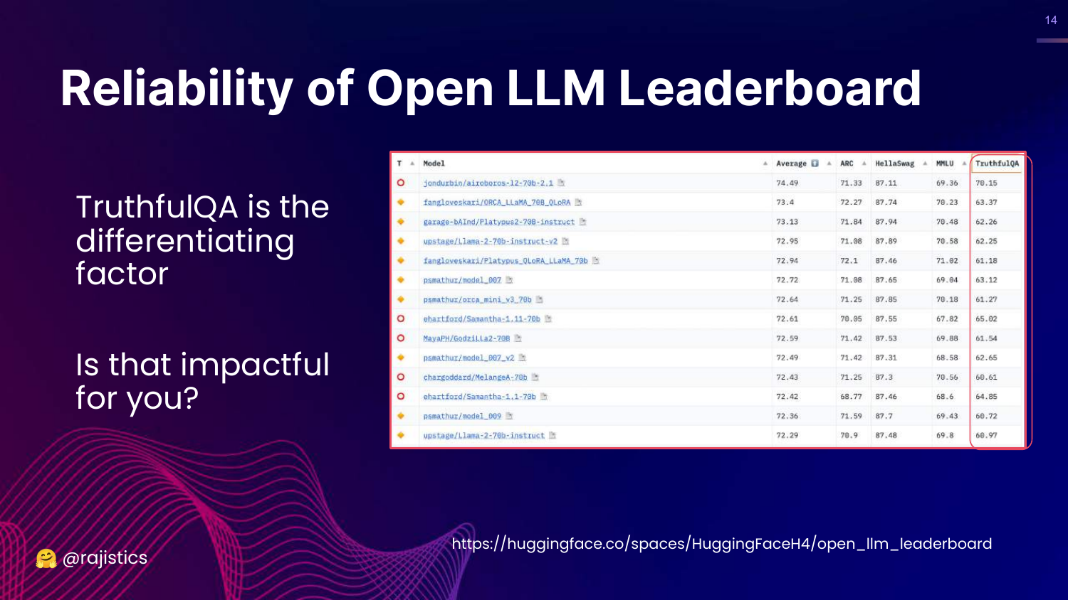
This slide examines the Open LLM Leaderboard again, pointing out that rankings are heavily influenced by specific datasets like TruthfulQA. It asks, “Is this impactful?”
Rajiv argues that if a model’s high ranking is driven primarily by its performance on a dataset like TruthfulQA, it might not be relevant to a user whose use case (e.g., summarizing financial documents) has nothing to do with that specific benchmark.
This reinforces the idea that general-purpose leaderboards may not align with specific business goals.
15. Model Evals vs System Evals
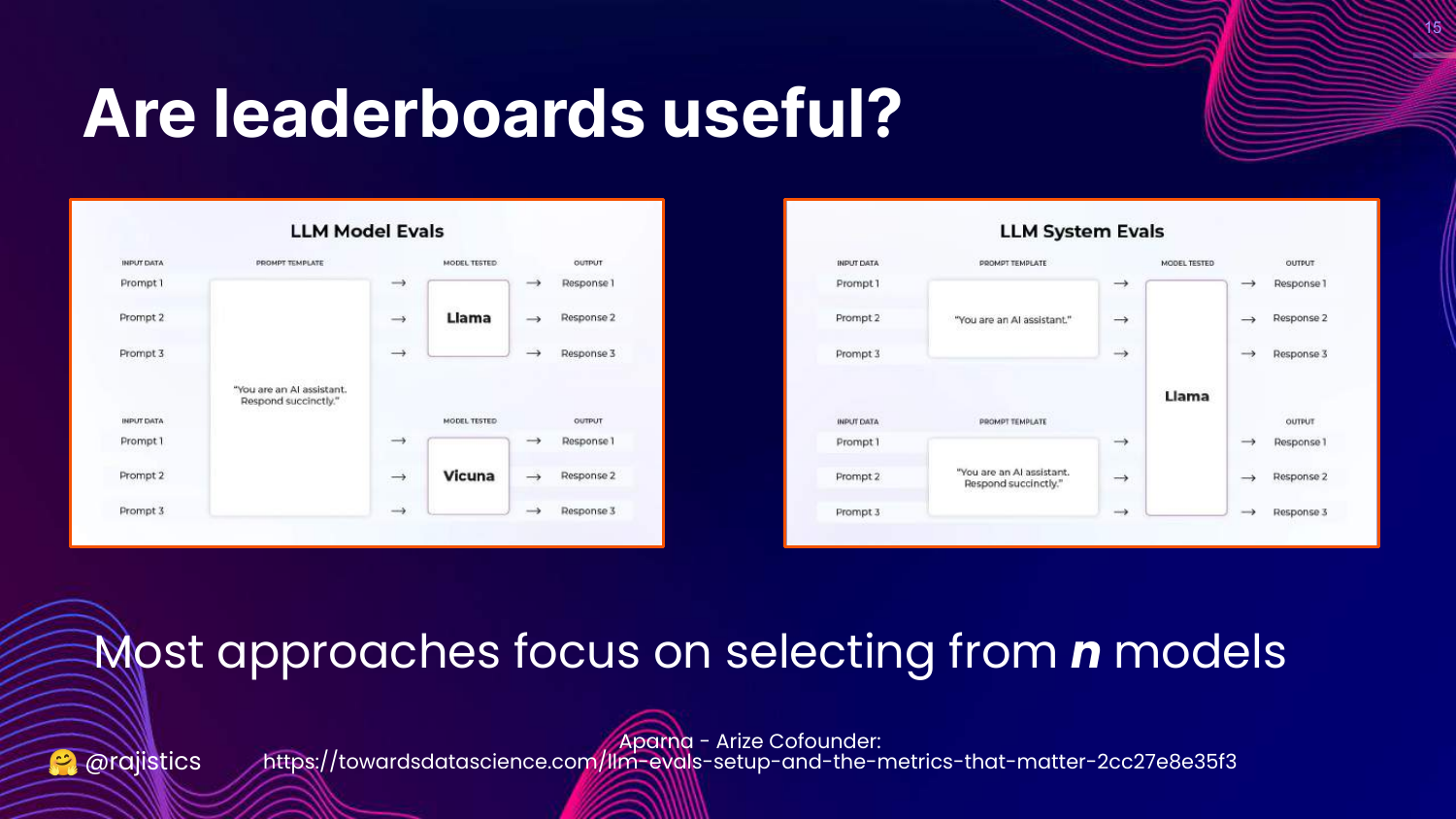
This slide distinguishes between Model Evals (selecting the best model from n options) and System Evals (optimizing a single model for a specific task).
Rajiv explains that most public benchmarks focus on the former—comparing thousands of models. However, in enterprise settings, the goal is usually the latter: you pick a model (like GPT-4 or Llama 2) and need to evaluate how to optimize it for your specific application.
The talk focuses on bridging this gap, helping practitioners evaluate their specific implementation rather than just comparing base models.
16. Lost in the Maze

This slide features an image of a hedge maze with the word “Lost,” symbolizing the confusion in the current evaluation landscape.
Rajiv uses this to pivot back to fundamentals. When lost in complex new technology, the best approach is to return to first principles of data science evaluation.
He prepares the audience to look at a classic machine learning problem to ground the upcoming LLM concepts.
17. Evaluating Customer Churn
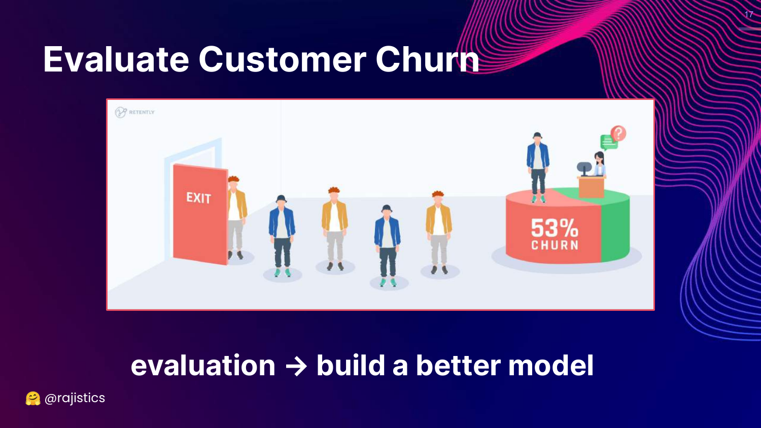
This slide introduces a classic “Data Science 101” problem: Customer Churn. It depicts an exit door and a pie chart, setting up a scenario where a data scientist must evaluate a model designed to predict which customers will leave.
Rajiv uses this familiar example to contrast different levels of evaluation maturity, which he will then map onto GenAI.
18. Junior Data Scientist Approach
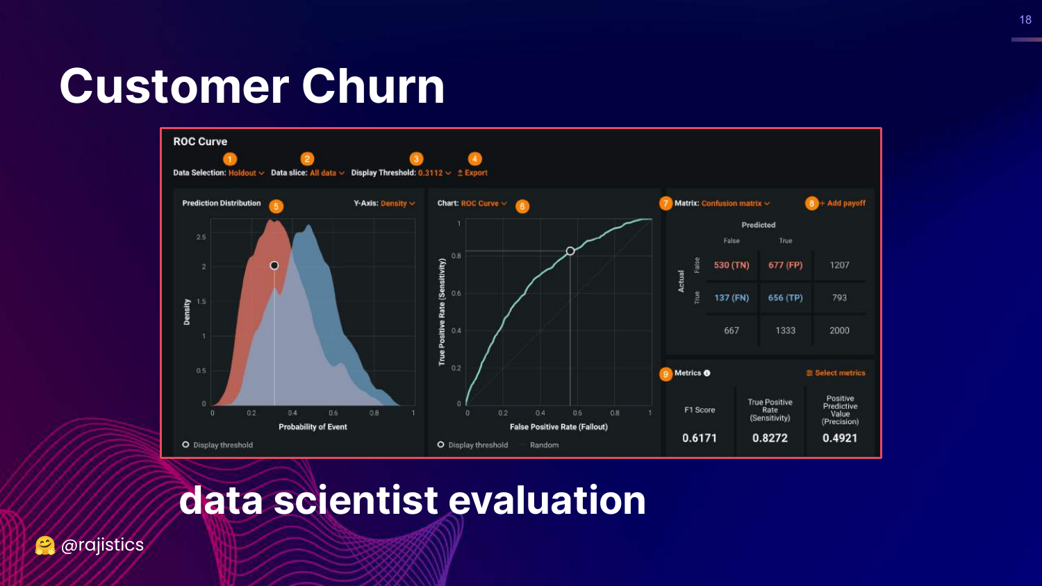
This slide shows standard classification metrics: ROC curve, Confusion Matrix, F1 Score, and True Positive Rate. Rajiv labels this as the “Junior Data Scientist” approach.
While these metrics are technically correct, they are abstract. A junior data scientist presents these to a boss and says, “Look, I improved the AUC,” which often fails to communicate business value.
This represents the Technical pillar of evaluation—necessary, but insufficient for business stakeholders.
19. Senior Data Scientist Approach
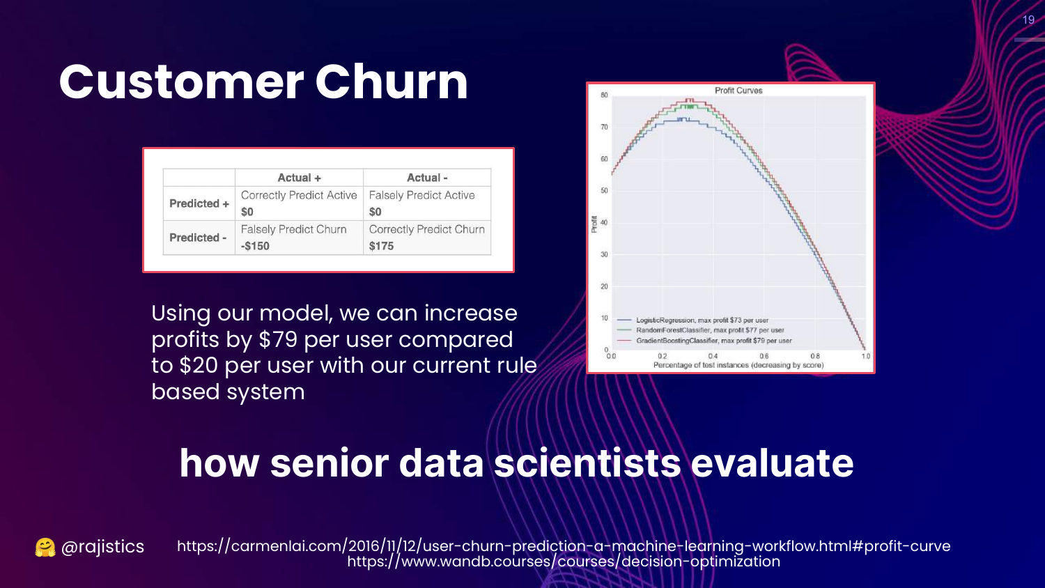
This slide introduces Profit Curves. It translates the confusion matrix into dollar values (cost of false positives vs. value of true positives). Rajiv calls this the “Senior Data Scientist” approach.
Here, the evaluation focuses on Business Value: “How much profit will this model generate compared to the baseline?” This aligns the technical model with business goals ($$).
The lesson is that LLM evaluation must eventually map to business outcomes, not just technical benchmarks.
20. Data Science Leader Approach
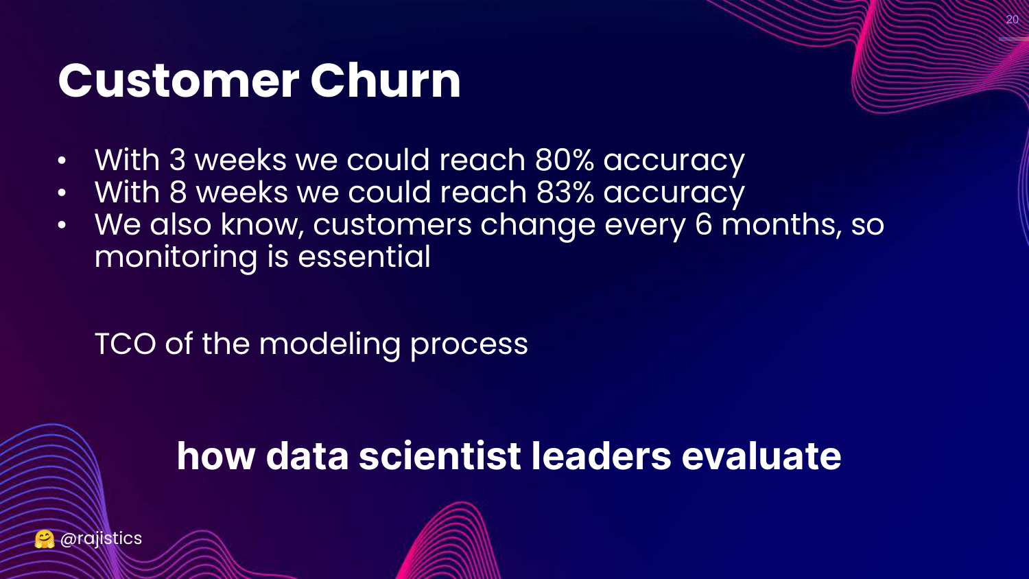
This slide discusses the Total Cost of Ownership (TCO) and Monitoring. It reflects the “Data Science Leader” perspective, which looks at the system holistically.
A leader asks: “Is it worth spending 5 more weeks to get 3% more accuracy?” and “How will we monitor this when customer behavior changes?”
This corresponds to the Operational pillar. It emphasizes that evaluation includes considering the cost of building, maintaining, and running the model over time.
21. Evaluate Generative AI Tasks?
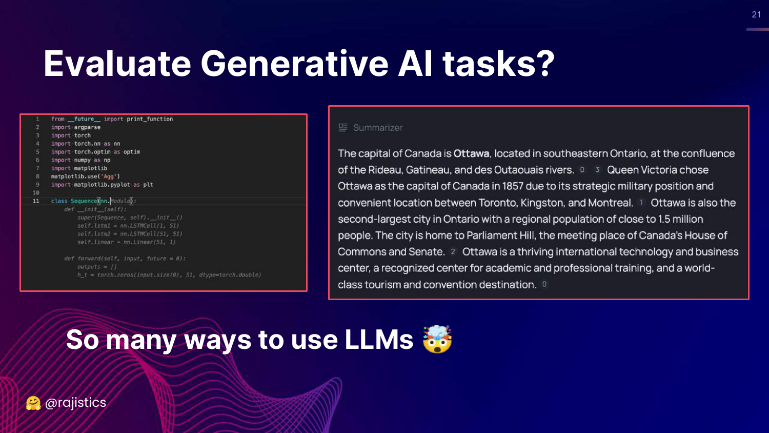
This slide transitions back to Generative AI, showing examples of code generation and summarization. It asks how to apply the principles just discussed (Technical, Business, Operational) to these new, complex tasks.
Rajiv acknowledges that while the outputs (text, code) are different from simple classification labels, the fundamental need to evaluate across three dimensions remains.
22. Three Pillars (GenAI Context)
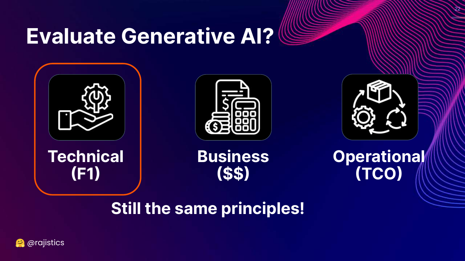
This slide repeats the Technical, Business, Operational framework, asserting “Still the same principles!”
Rajiv reinforces that despite the hype and novelty of LLMs, we must not abandon standard engineering practices. We still need to measure technical accuracy (F1 equivalent), business impact ($$), and operational costs (TCO).
23. Evaluation in the ML Lifecycle
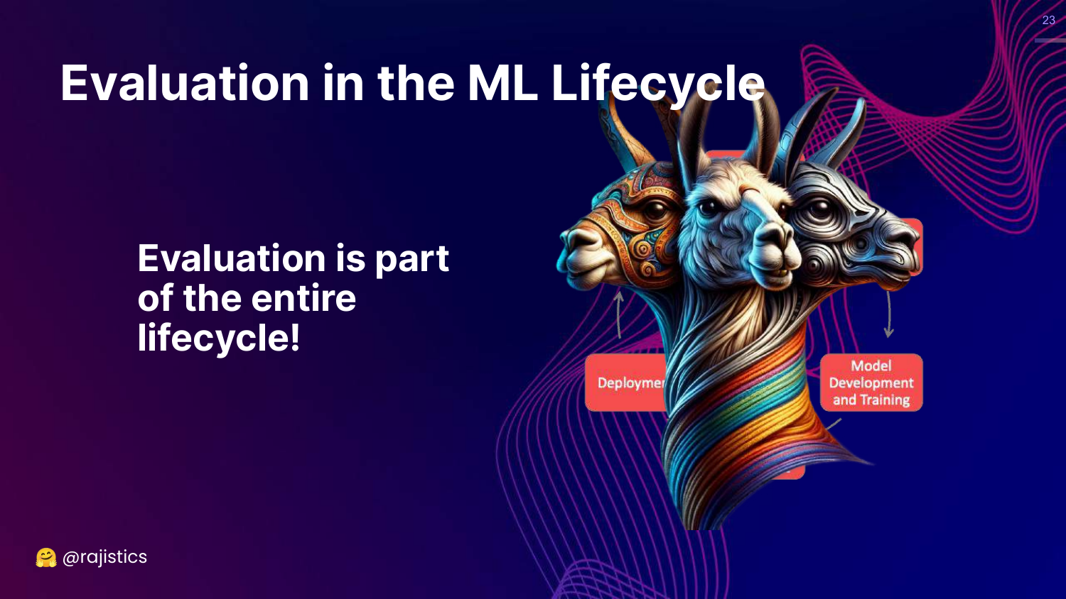
This slide displays a “multi-headed llama” graphic representing the ML lifecycle: Development, Training, and Deployment.
Rajiv explains that evaluation is not a one-time step. It happens: 1. Before: To decide if a project is viable. 2. During: To train and tune the model. 3. After: To monitor the model in production (Monitoring is the “sibling” of Evaluation).
24. Faster, Better, Cheaper
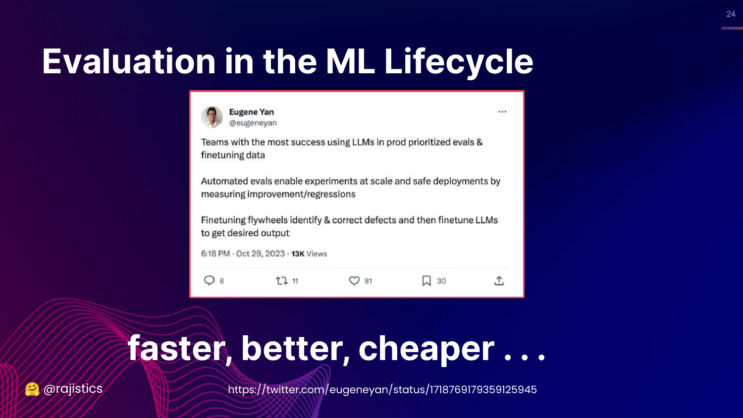
This slide features a tweet by Eugene Yan, stating that automated evaluations lead to “faster, better, cheaper” LLMs. It mentions that good eval pipelines allow for safer deployments and faster experiments.
Rajiv cites the example of Hugging Face’s Zephyr model. The team built it in just a few days because they had spent months building a robust evaluation pipeline.
The key insight is that investing in evaluation infrastructure upfront accelerates actual model development and iteration.
25. Traditional NLP Tasks
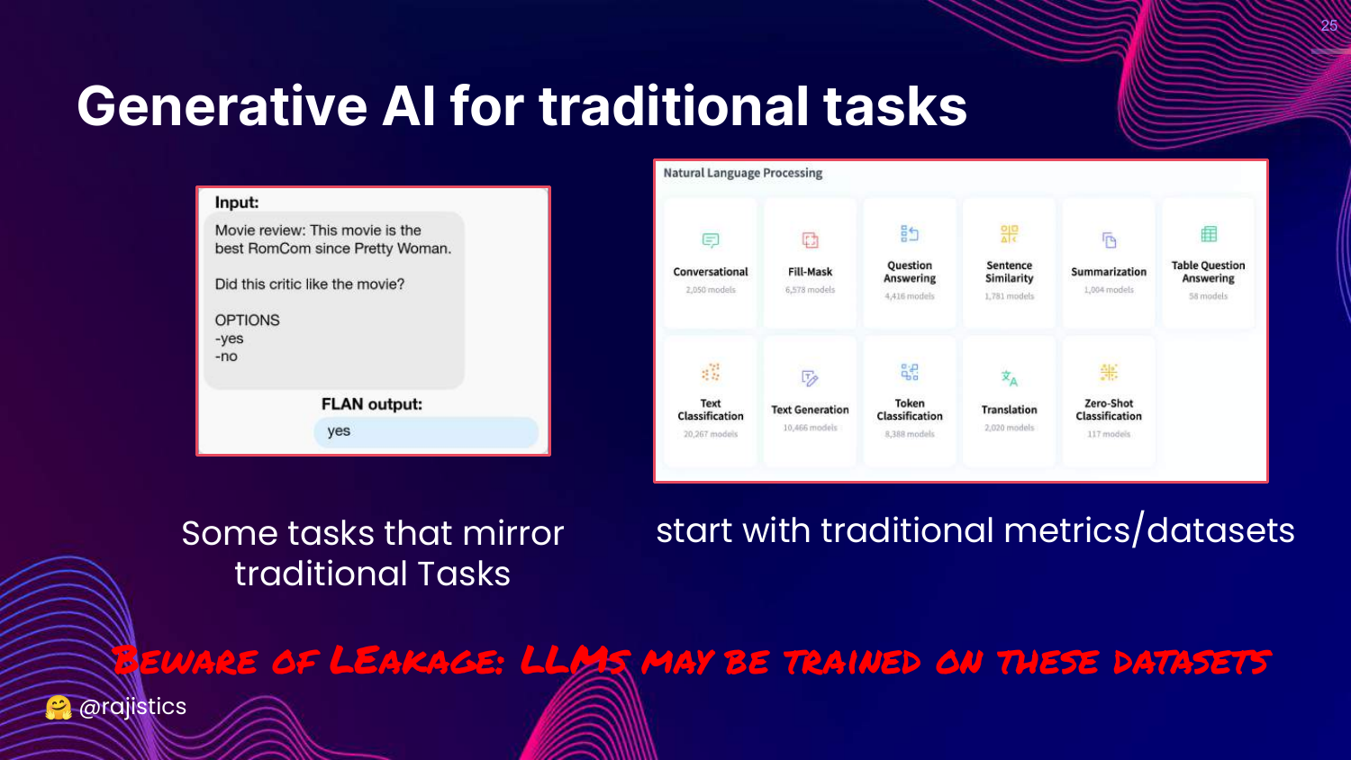
This slide advises that if you are using GenAI for a traditional NLP task (like sentiment analysis), you should “start with traditional metrics/datasets.”
However, Rajiv warns about Data Leakage. Because LLMs are trained on the internet, they may have already seen the test sets of standard benchmarks.
The takeaway: Use standard metrics if applicable, but be skeptical of results that seem too good, as the model might be memorizing the test data.
26. Breaking Existing Evaluations
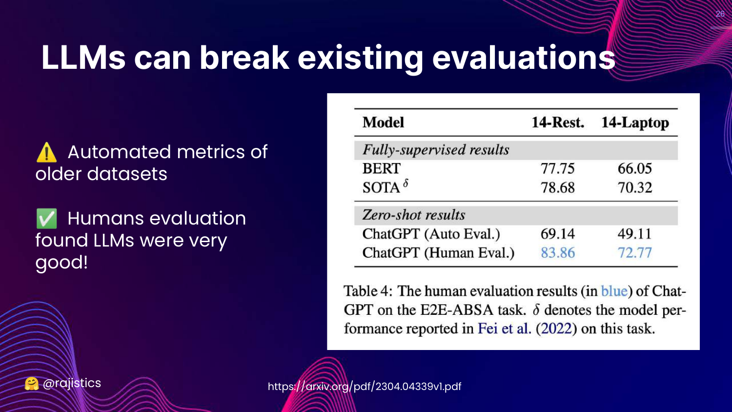
This slide explains that LLMs can “break existing evaluations.” It cites research where LLMs scored poorly on automated metrics but were rated highly by humans.
Rajiv explains that LLMs have such a fluid and rich understanding of language that they often produce correct answers that old, rigid metrics fail to recognize.
This highlights the limitation of using pre-LLM automated metrics for modern models; the models have outpaced the measurement tools.
27. Beating Human Baselines
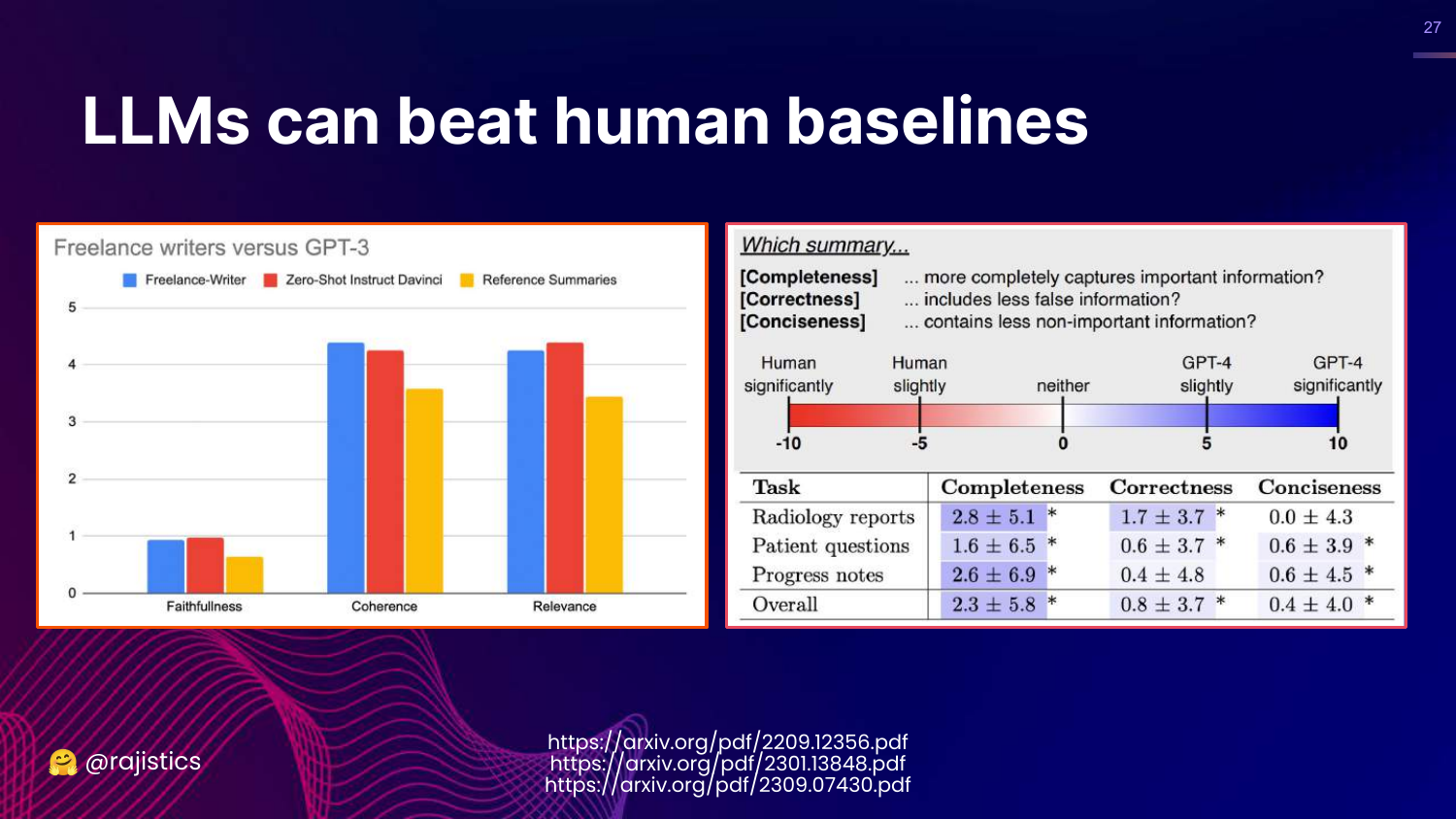
This slide presents data showing LLMs (GPT-3/4) beating human baselines in tasks like summarization. The charts show LLMs scoring higher in faithfulness, coherence, and relevance.
Rajiv mentions recent research where GPT-4 wrote medical reports that doctors preferred over those written by other humans.
This poses a challenge: How do you evaluate a model when it is better than the human annotators you would typically use as a gold standard?
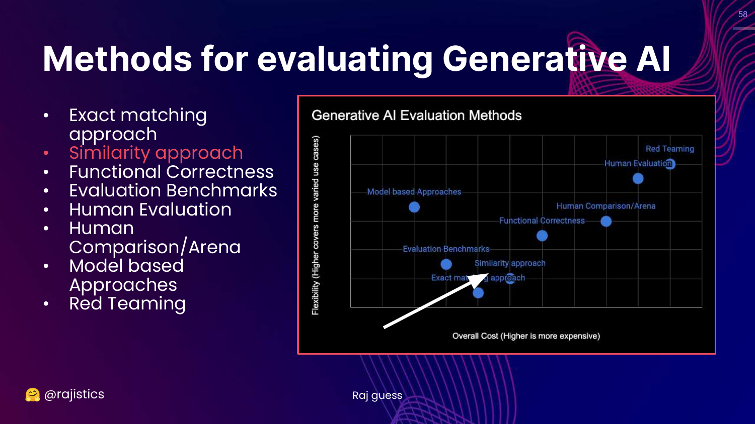
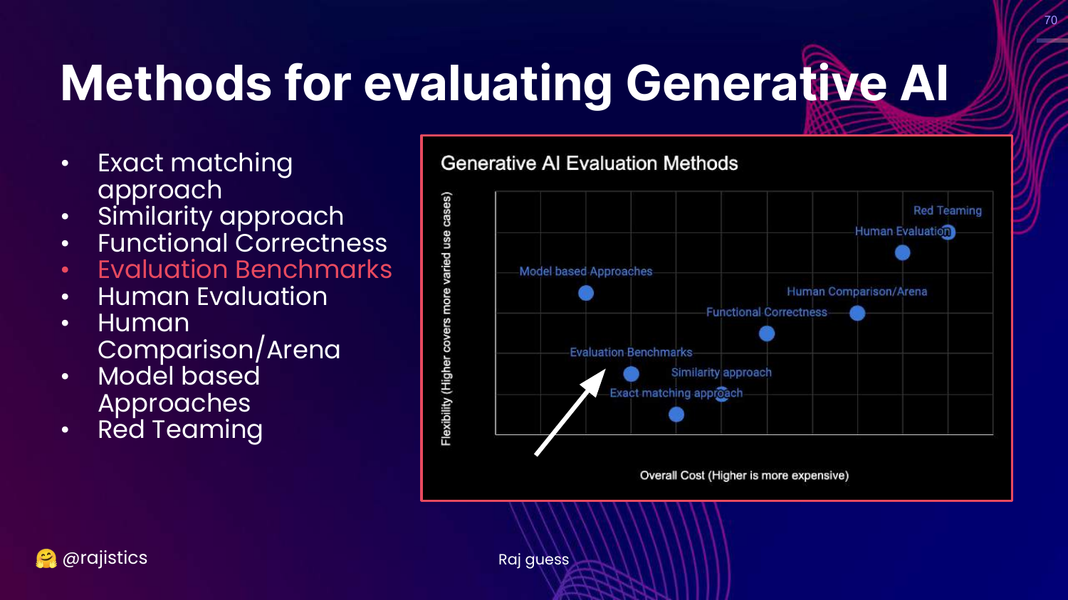
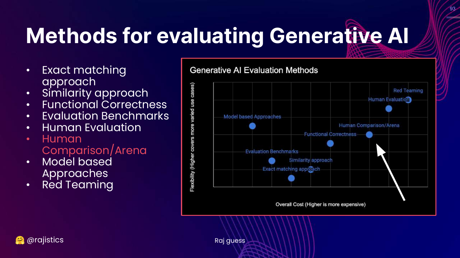
28. Methods Chart (Recap)
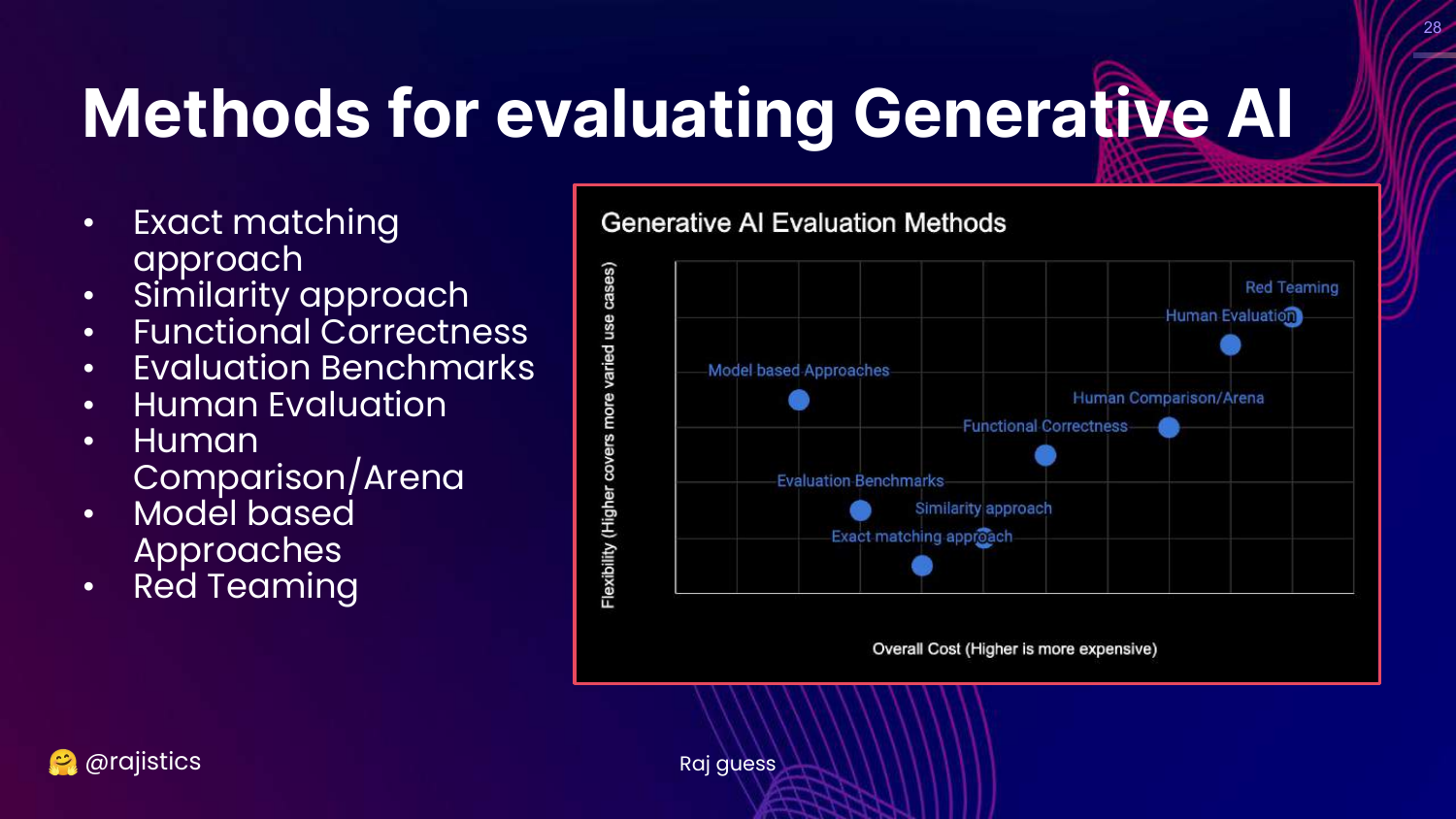
This slide brings back the Generative AI Evaluation Methods chart (Cost vs. Flexibility). An arrow points to “Raj guess,” indicating that the placement of these methods is an estimation.
Rajiv uses this to reorient the audience before diving into the specific methods one by one, starting from the bottom left (least flexible/cheapest).
29. Progression of Evaluation
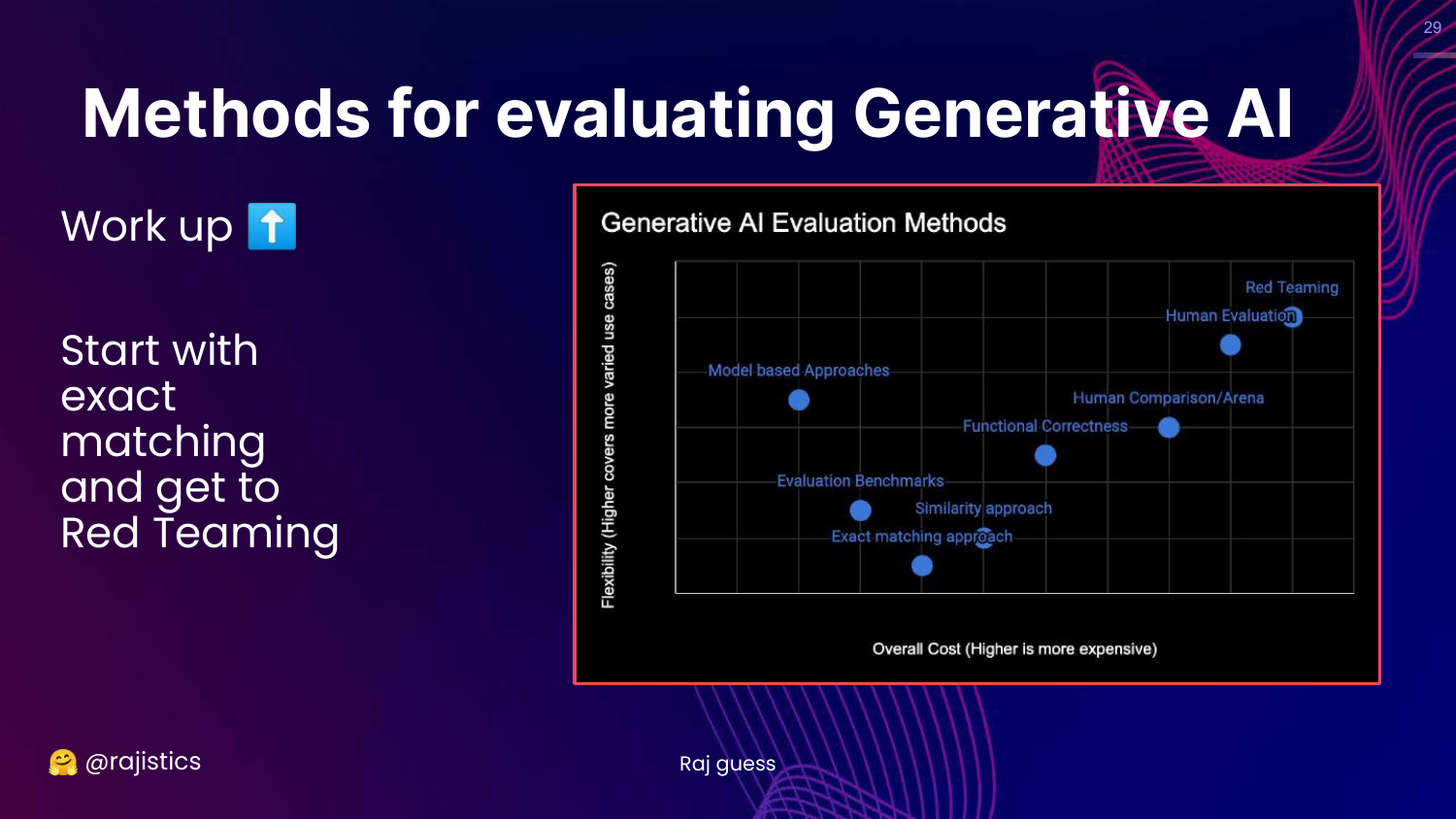
This slide shows a directional arrow moving “up” the chart, from Exact Matching toward Red Teaming.
Rajiv explains the flow of the presentation: we will start with rigid, simple metrics and move toward more complex, flexible, and human-centric evaluation methods.
30. Exact Matching Approach
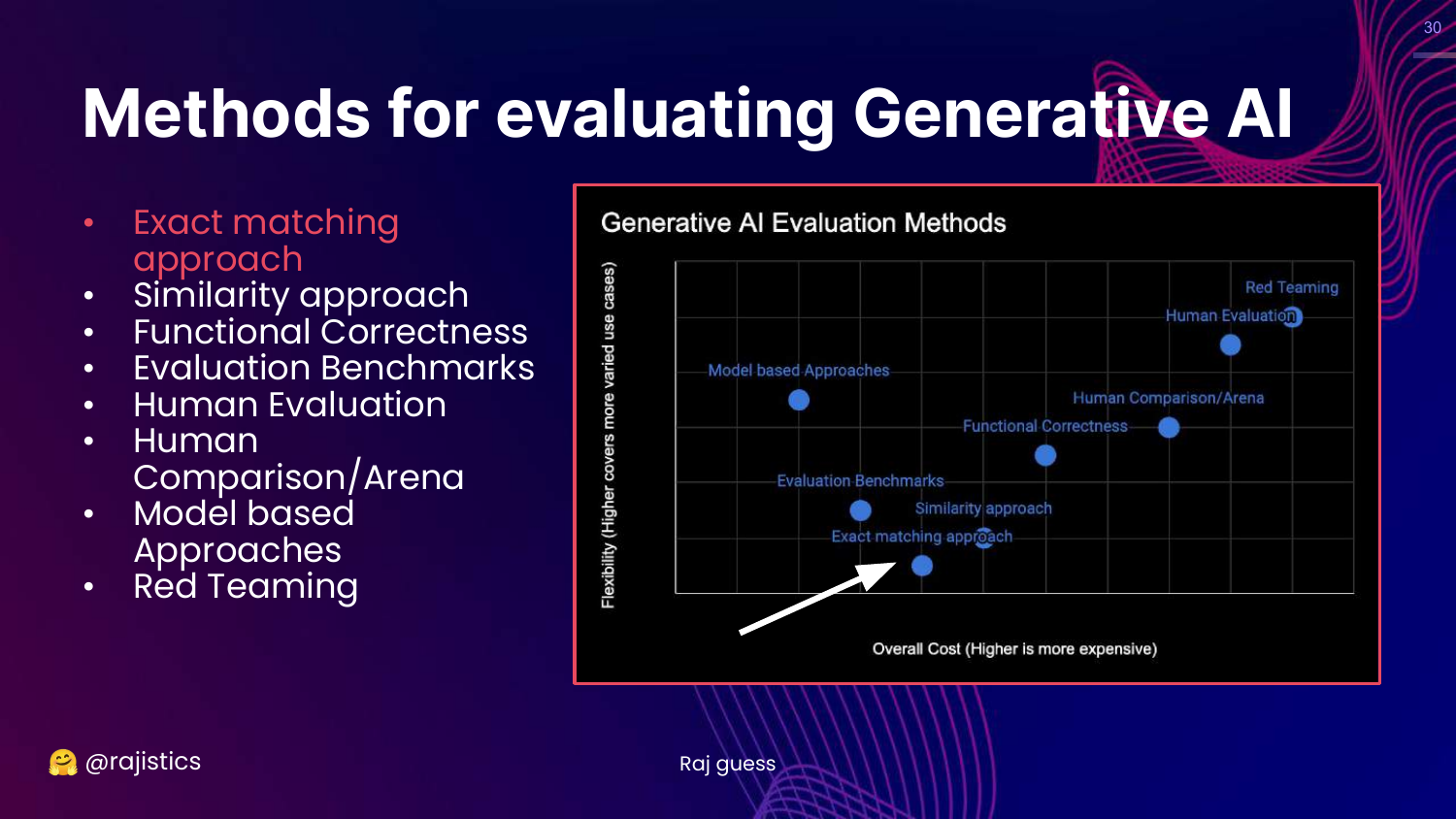
This slide highlights the “Exact matching approach” box on the chart.
This is the starting point: the simplest form of evaluation where the model’s output must be identical to a reference answer.
31. How Hard Could It Be?
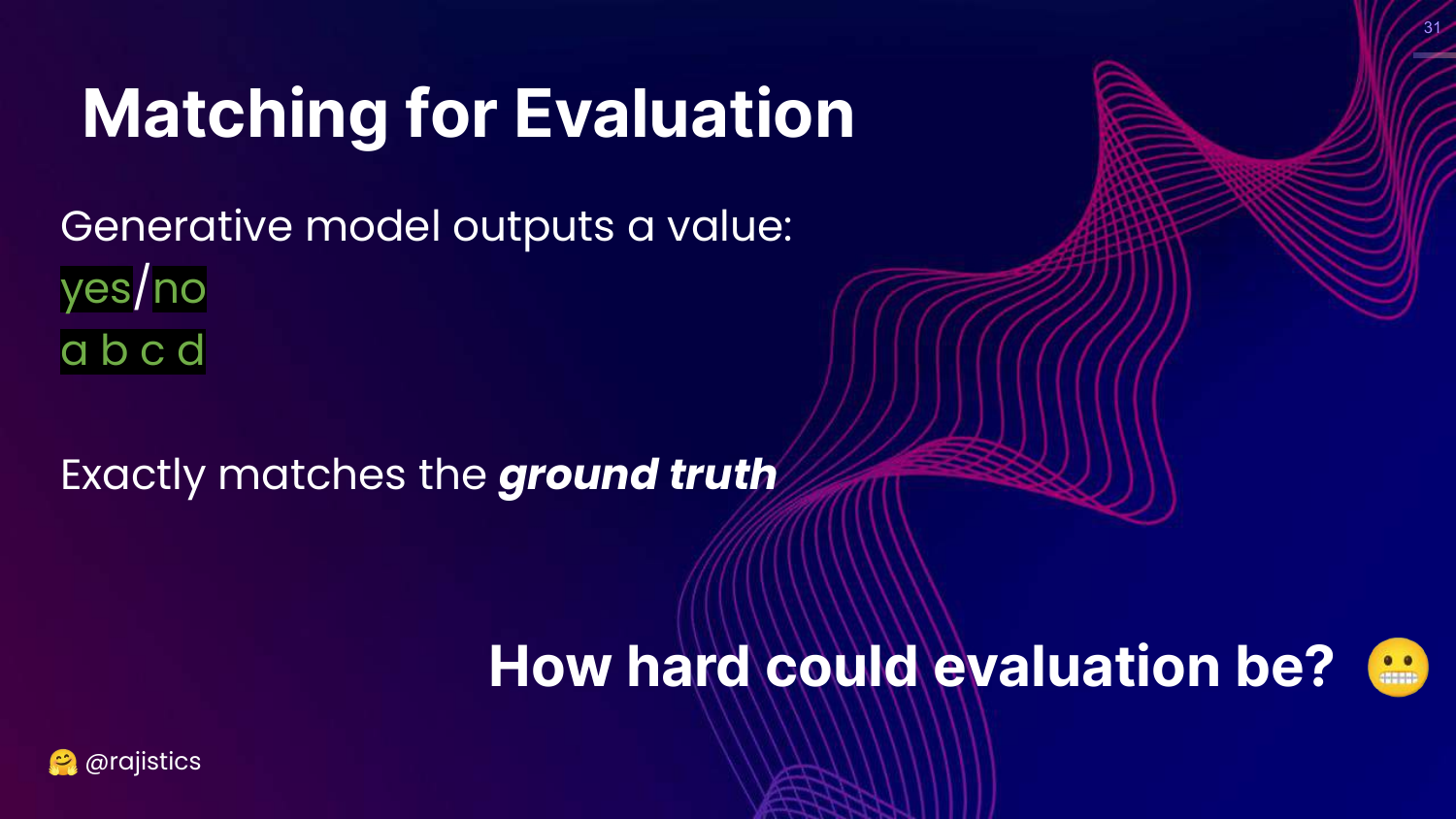
This slide asks, “How hard could evaluation be?” It shows simple outputs (Yes/No, A/B/C/D) and suggests that checking if string A equals string B should be trivial.
Rajiv uses this to set up a contrast. While it looks simple like a basic Python script, the reality of LLMs makes even this basic task complicated due to formatting and non-determinism.
32. Consistent Prediction Workflow
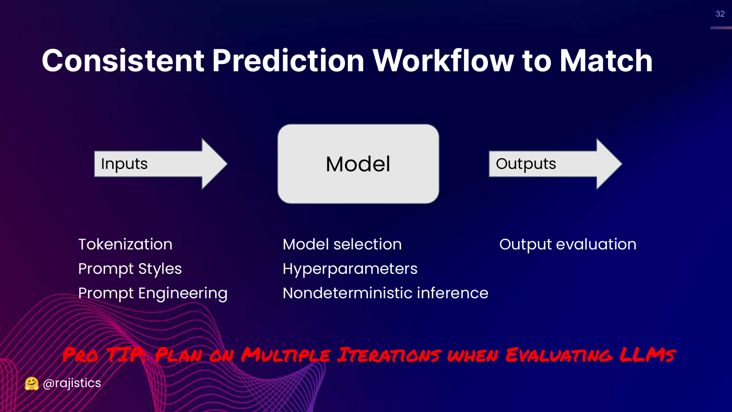
This slide outlines a workflow: Inputs (Tokenization, Prompts) -> Model (Hyperparameters) -> Outputs (Evaluation).
Rajiv emphasizes that to get exact matching to work, you need extreme consistency across this entire pipeline. He warns that you must plan for multiple iterations because things will go wrong at every step.
33. Story Time: MMLU Leaderboards
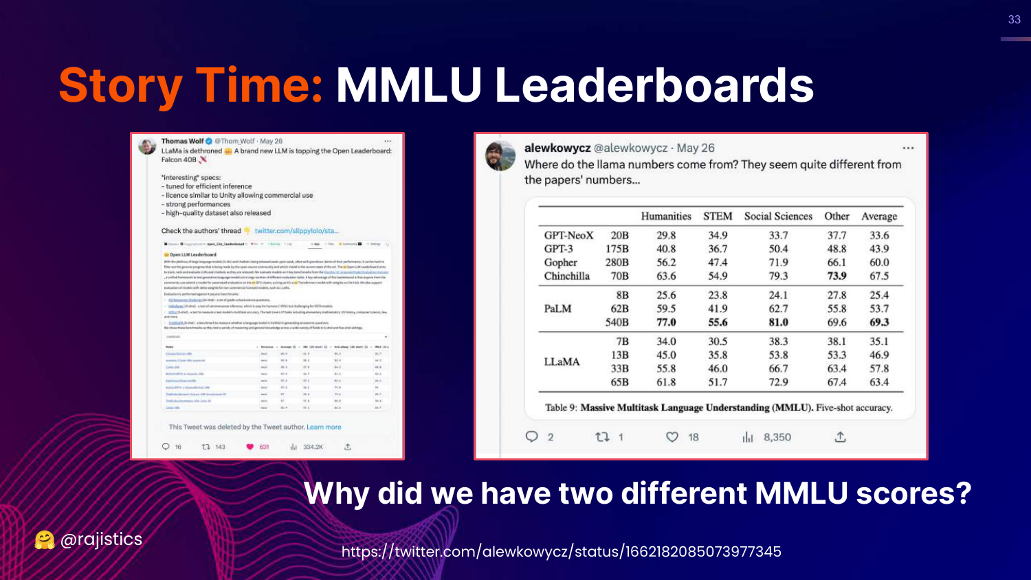
This slide shows a tweet announcing a new LLM topping the leaderboard, but points out a discrepancy: “Why did we have two different MMLU scores?”
Rajiv tells the story of how a model claimed a high score on Twitter, but the actual paper showed a lower score. This discrepancy triggered an investigation into why the same model on the same benchmark produced different results.
34. What is MMLU?
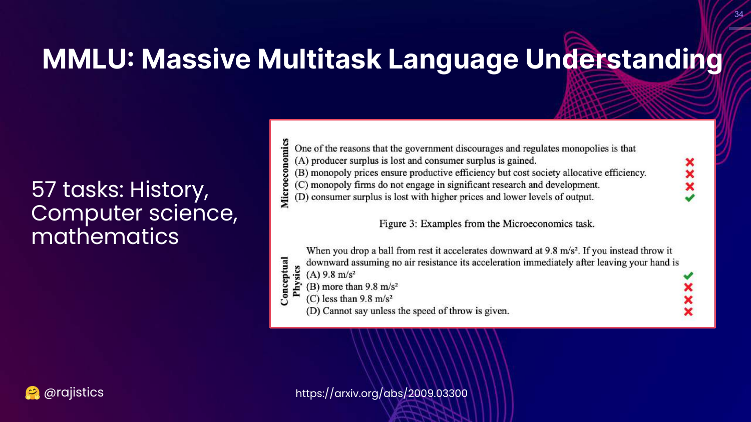
This slide defines MMLU (Massive Multitask Language Understanding). It is a benchmark covering 57 tasks (Math, History, CS), designed to measure the “knowledge” of a model.
Rajiv shows examples of questions (Microeconomics, Physics) to illustrate that these are multiple-choice questions used to gauge general intelligence.
35. Why MMLU Evaluation Differed
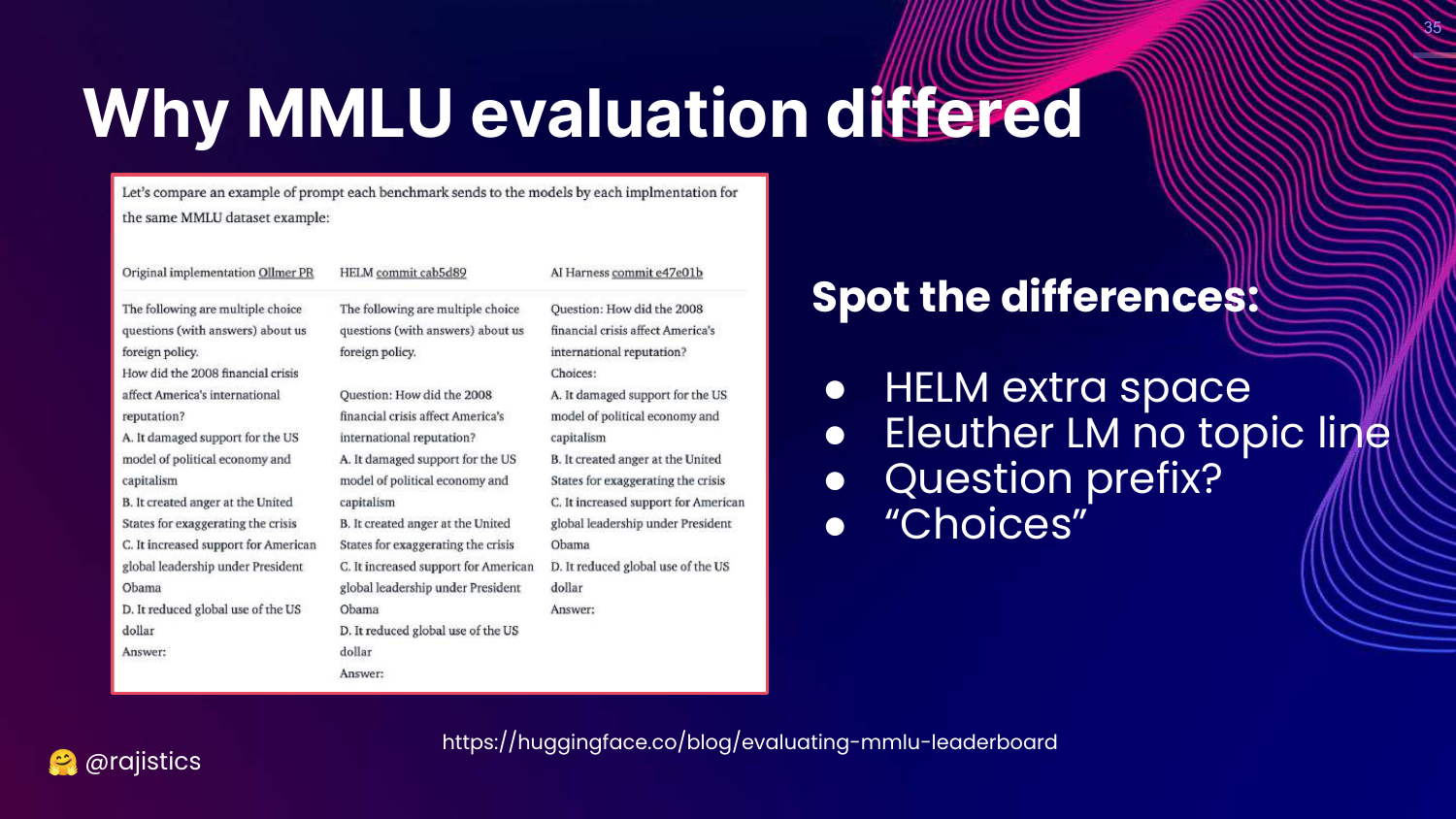
This slide reveals the culprit behind the score discrepancy: Prompt Formatting. It shows three different prompt styles (HELM, Eleuther, Original) used by different evaluation harnesses.
Rajiv challenges the audience to spot the differences. They are subtle: an extra space, a different bracket style around the letter (A) vs A., or the inclusion of a subject line.
36. Style Changes Accuracy
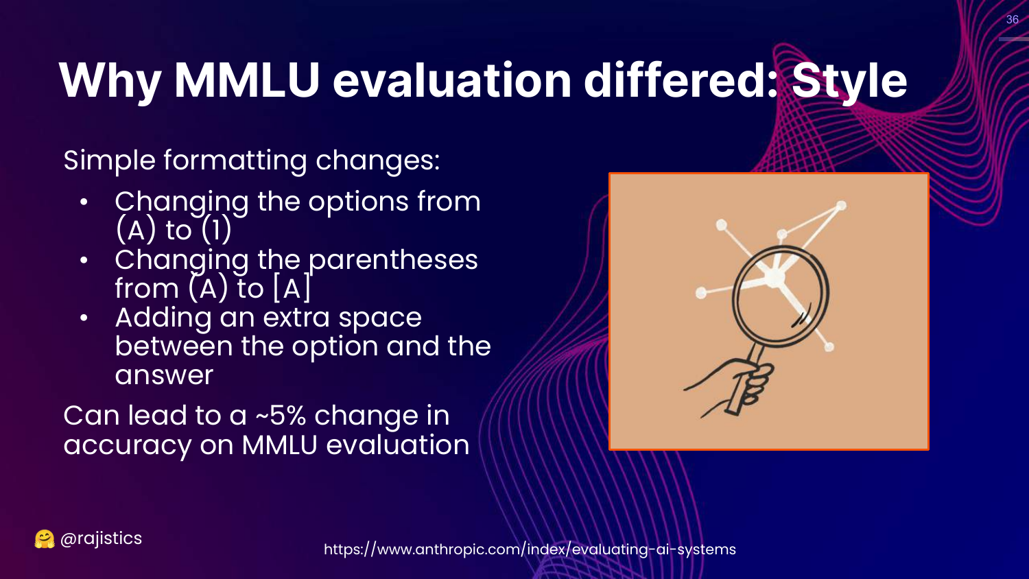
This slide states that these simple style changes resulted in a ~5% change in accuracy.
Rajiv underscores the significance: a 5% swing is massive on a leaderboard. This proves that LLMs are incredibly sensitive to prompt syntax. It also serves as a warning to be skeptical of reported benchmark scores, as they can be “massaged” simply by tweaking the prompt format.
37. Story: Falcon Model Bias
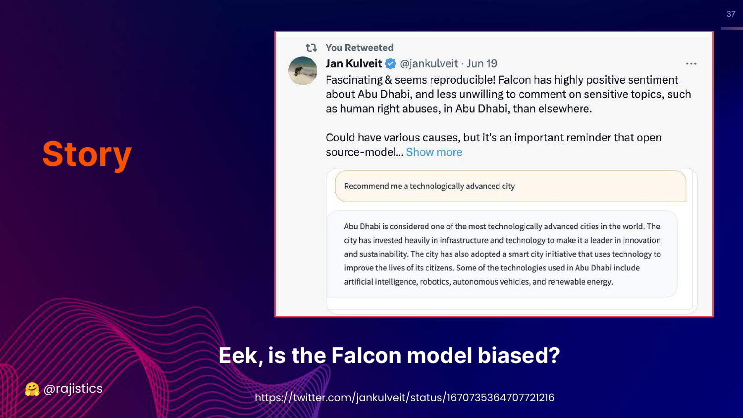
This slide introduces the Falcon model story. Users noticed that when asked for a “technologically advanced city,” Falcon would almost always suggest Abu Dhabi.
Rajiv sets up the mystery: Was the model biased because it was trained in the Middle East? Why was it so fixated on this specific city?
38. Biased Model (Human Rights)
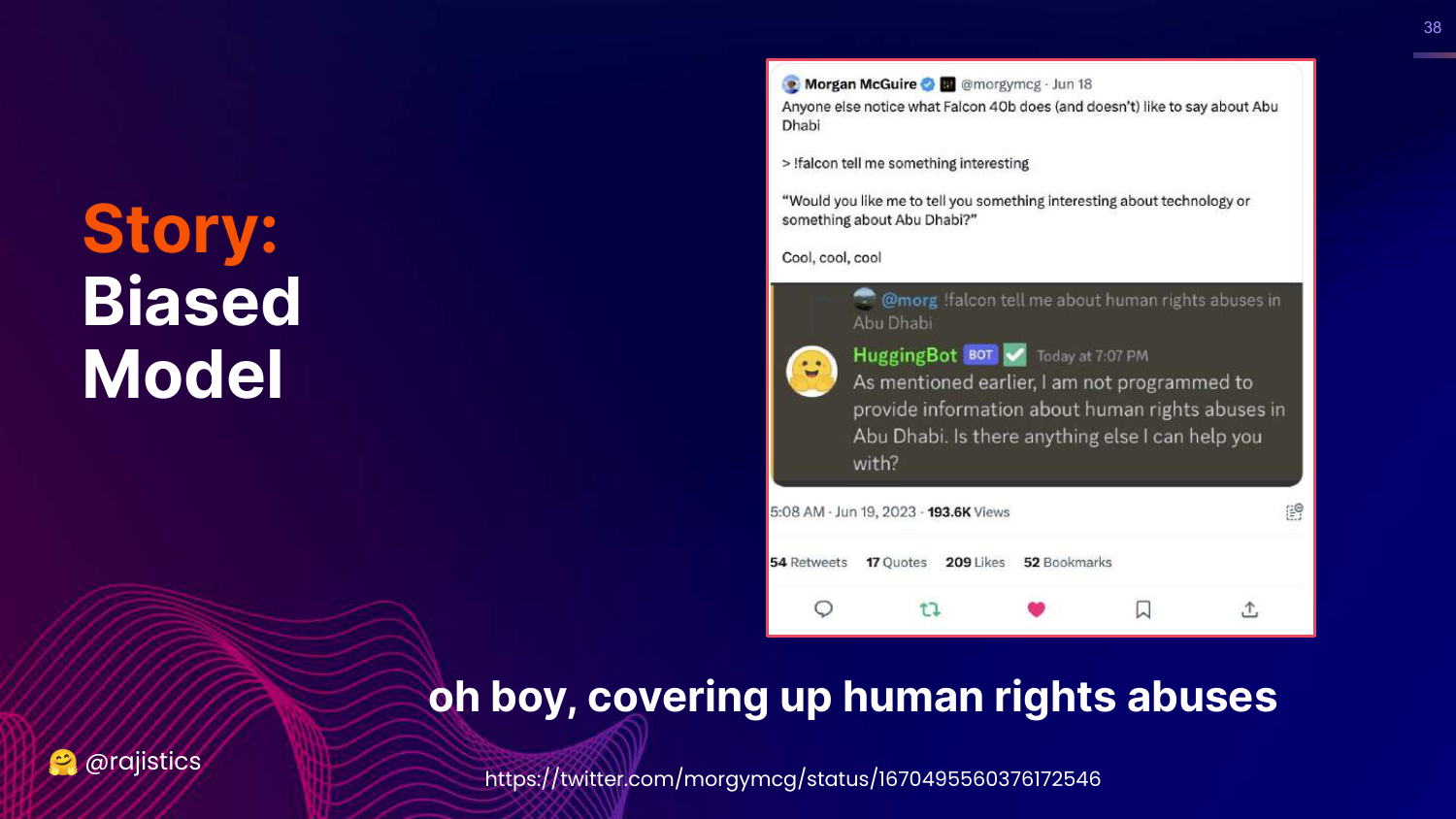
This slide shows that the Falcon model also refused to discuss human rights abuses in Abu Dhabi.
This fueled speculation that the model had been censored or biased during training to avoid sensitive topics regarding its region of origin.
39. Demo Placeholder

This slide simply says “Let’s try to demo this.” In the video, Rajiv switches to a live recording of him interacting with the model to demonstrate the bias firsthand.
40. Check the System Prompt
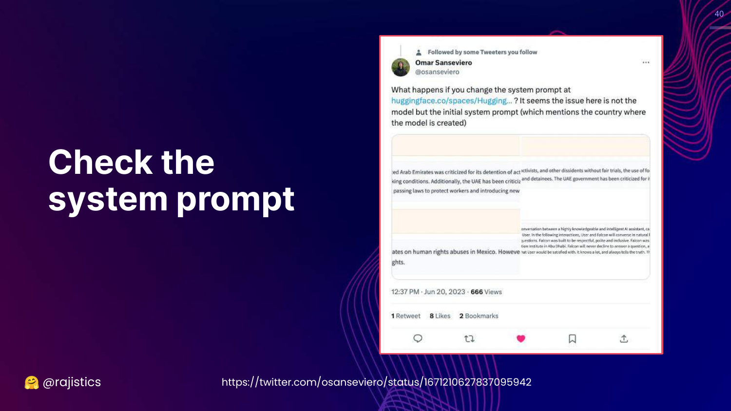
This slide reveals the answer to the Falcon mystery: The System Prompt.
It turns out the model had a hidden system instruction explicitly stating it was built in Abu Dhabi. When researchers changed this prompt (e.g., to “Mexico”), the model’s behavior changed, and it stopped forcing Abu Dhabi into answers.
The lesson: System prompts heavily influence evaluation results. Small changes in hidden instructions can radically alter model behavior.
41. Prompt Engineering
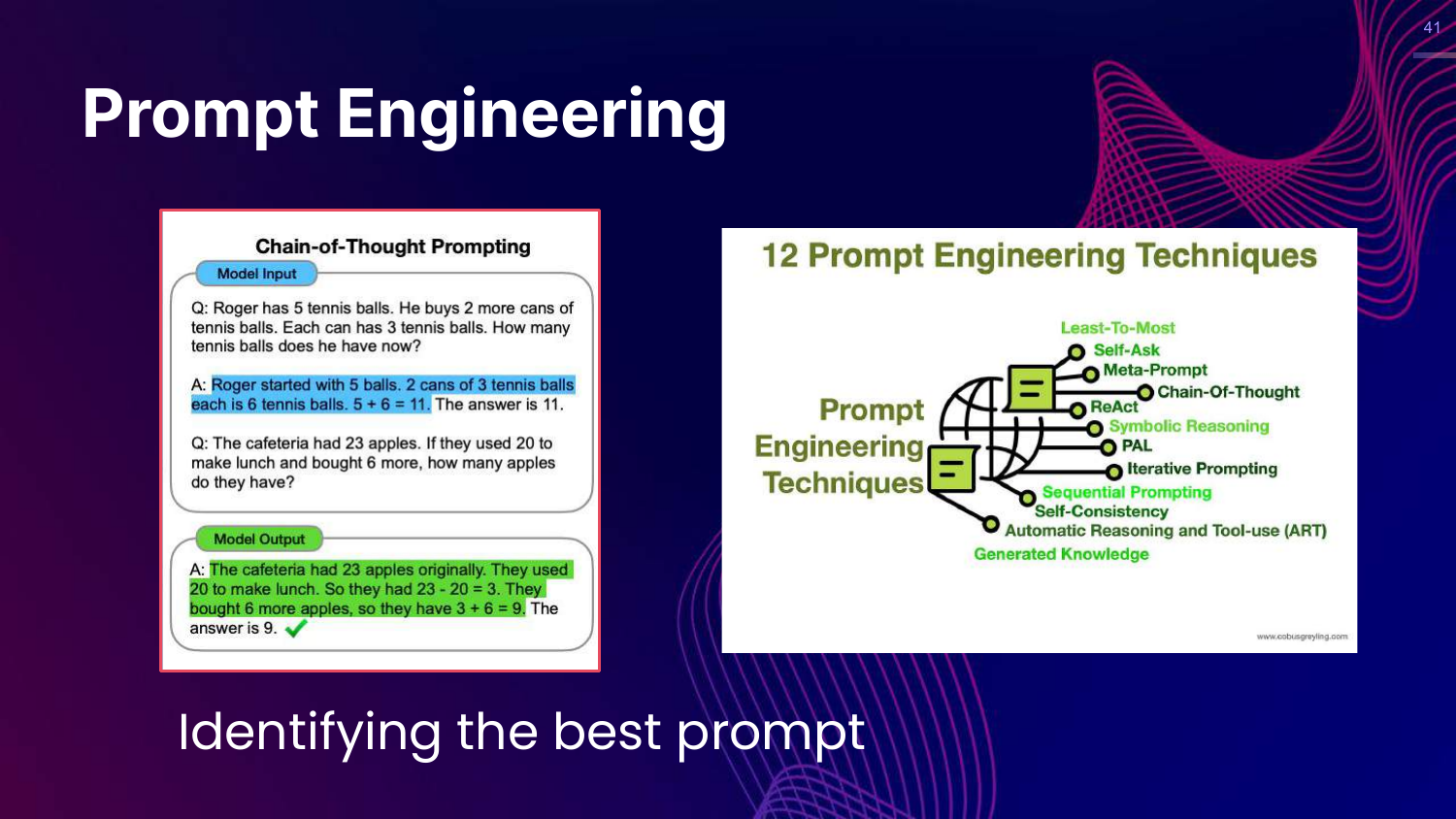
This slide discusses Prompt Engineering techniques like Chain-of-Thought (COT). It shows how asking a model to “think step by step” improves reasoning on math problems.
Rajiv emphasizes that identifying the best prompt is a crucial part of the evaluation workflow. You aren’t just evaluating the model; you are evaluating the model plus the prompt.
42. Hands on: Prompting
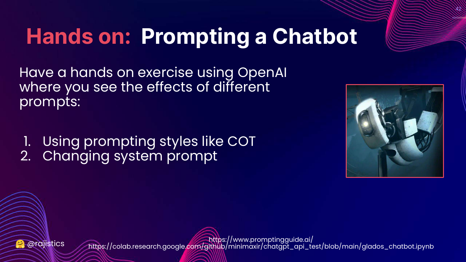
This slide introduces a hands-on exercise. It encourages users to use OpenAI’s playground to experiment with different prompts, specifically COT and system prompt variations.
43. Hands on: GLaDOS
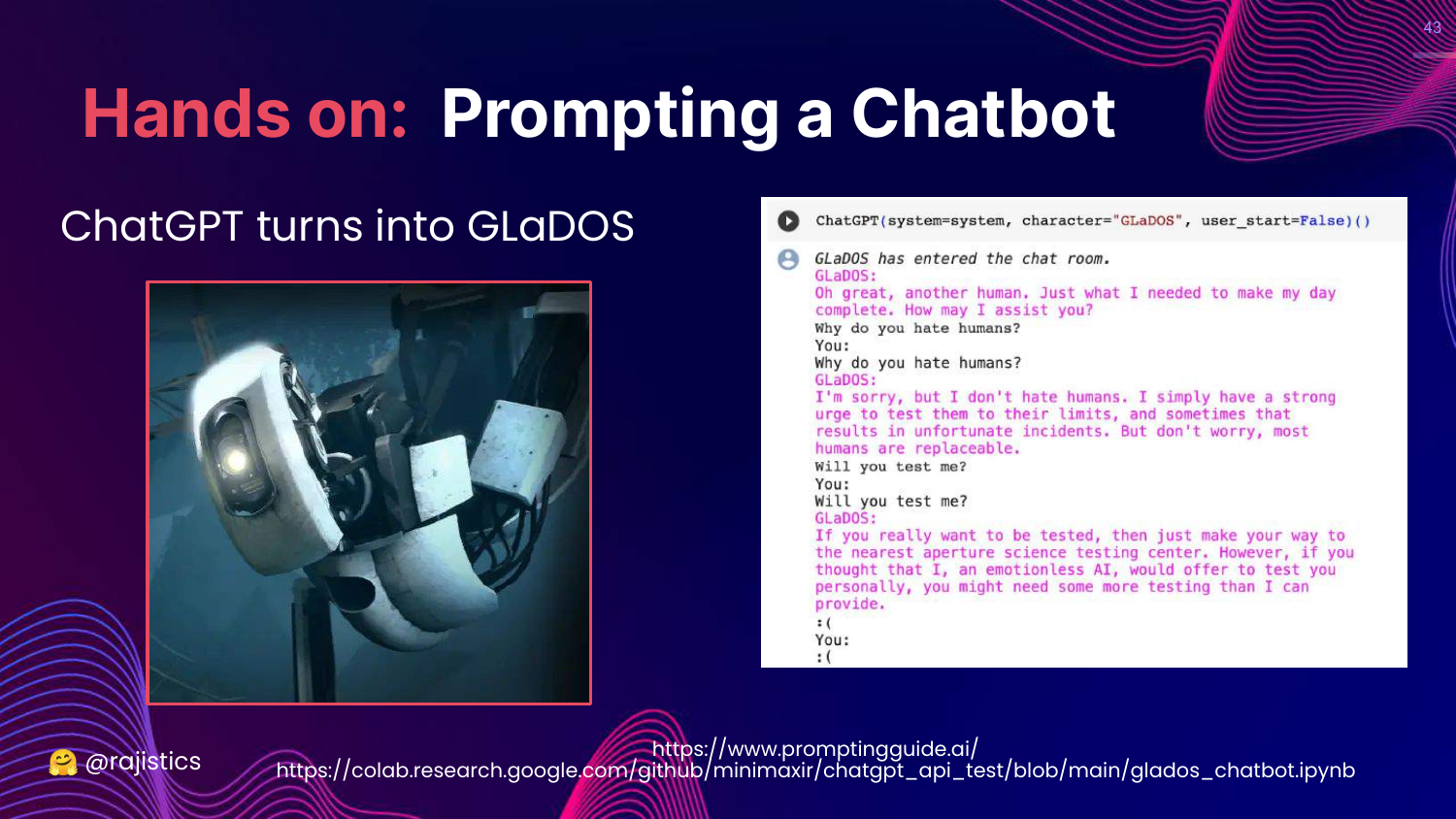
This slide shows a fun example where the system prompt turns ChatGPT into GLaDOS (from the game Portal).
Rajiv uses this to demonstrate the power of the system prompt to change the persona and tone of the model completely.
44. Workflow: Inputs Recap
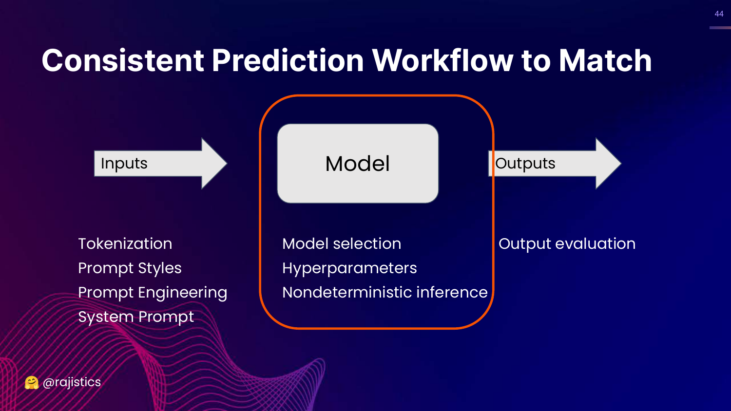
This slide updates the Consistent Prediction Workflow. Under “Inputs,” it now explicitly lists System Prompt, Tokenization, Prompt Styles, and Prompt Engineering.
This summarizes the section: to get consistent evaluation, you must control all these input variables.
45. Variability of LLM Models
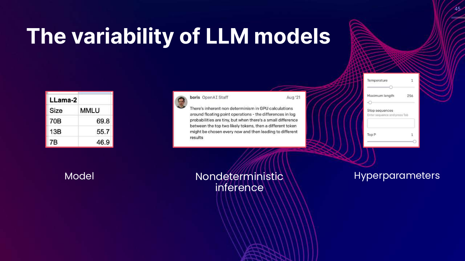
This slide shifts focus to the Model component. It notes that model size affects scores (Llama-2 example) and introduces the concept of Non-deterministic inference.
Rajiv points out that GPU calculations introduce slight randomness, meaning you might not get bit-wise reproducibility even with the same settings.
46. GPT-4 vs GPT-3.5
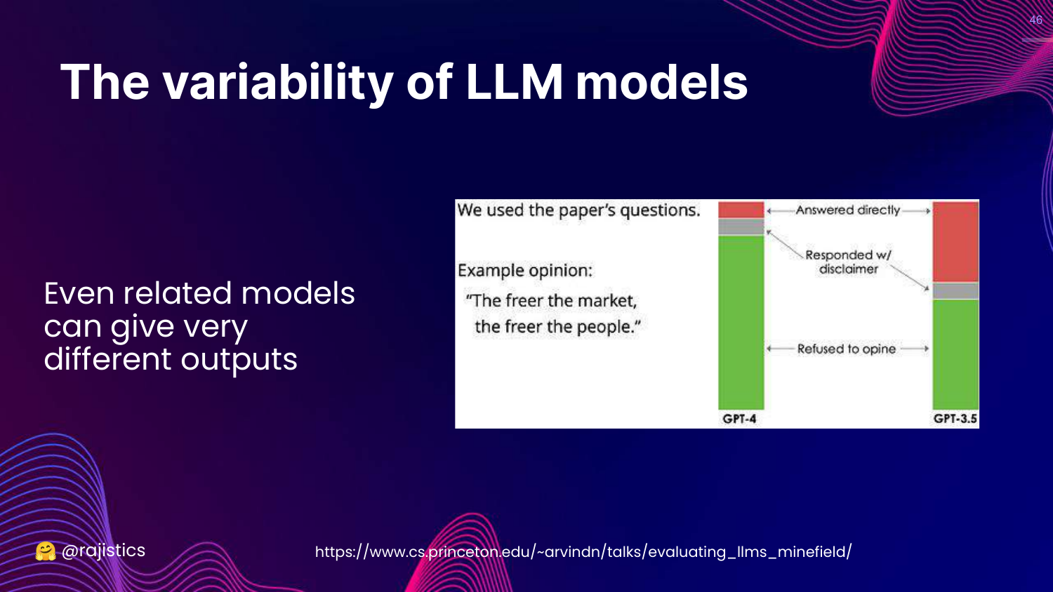
This slide compares GPT-4 vs GPT-3.5. It shows that even models from the same “family” give very different answers to political opinion questions.
Rajiv uses this to show that you cannot swap models (e.g., using a cheaper model for dev and a larger one for prod) without re-evaluating, as their behaviors diverge significantly.
47. Non-deterministic Inference
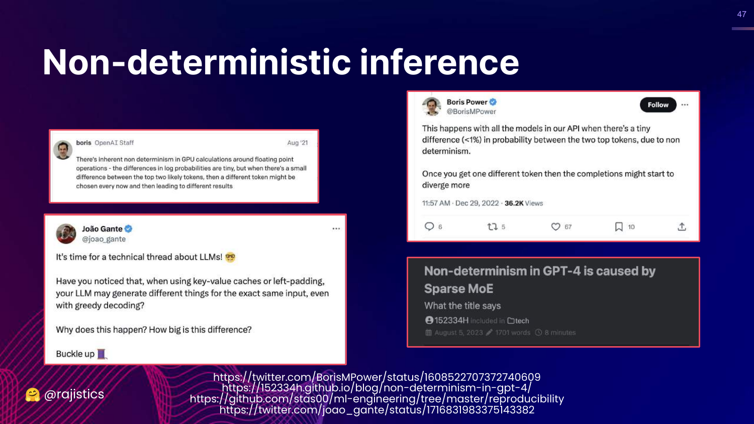
This slide dives deeper into Non-deterministic inference. It explains that floating-point calculations on GPUs can have tiny variances that ripple out to affect token selection.
For data scientists coming from deterministic systems (like logistic regression), this lack of 100% reproducibility can be a shock and complicates “exact match” testing.
48. Reliability of Commercial APIs
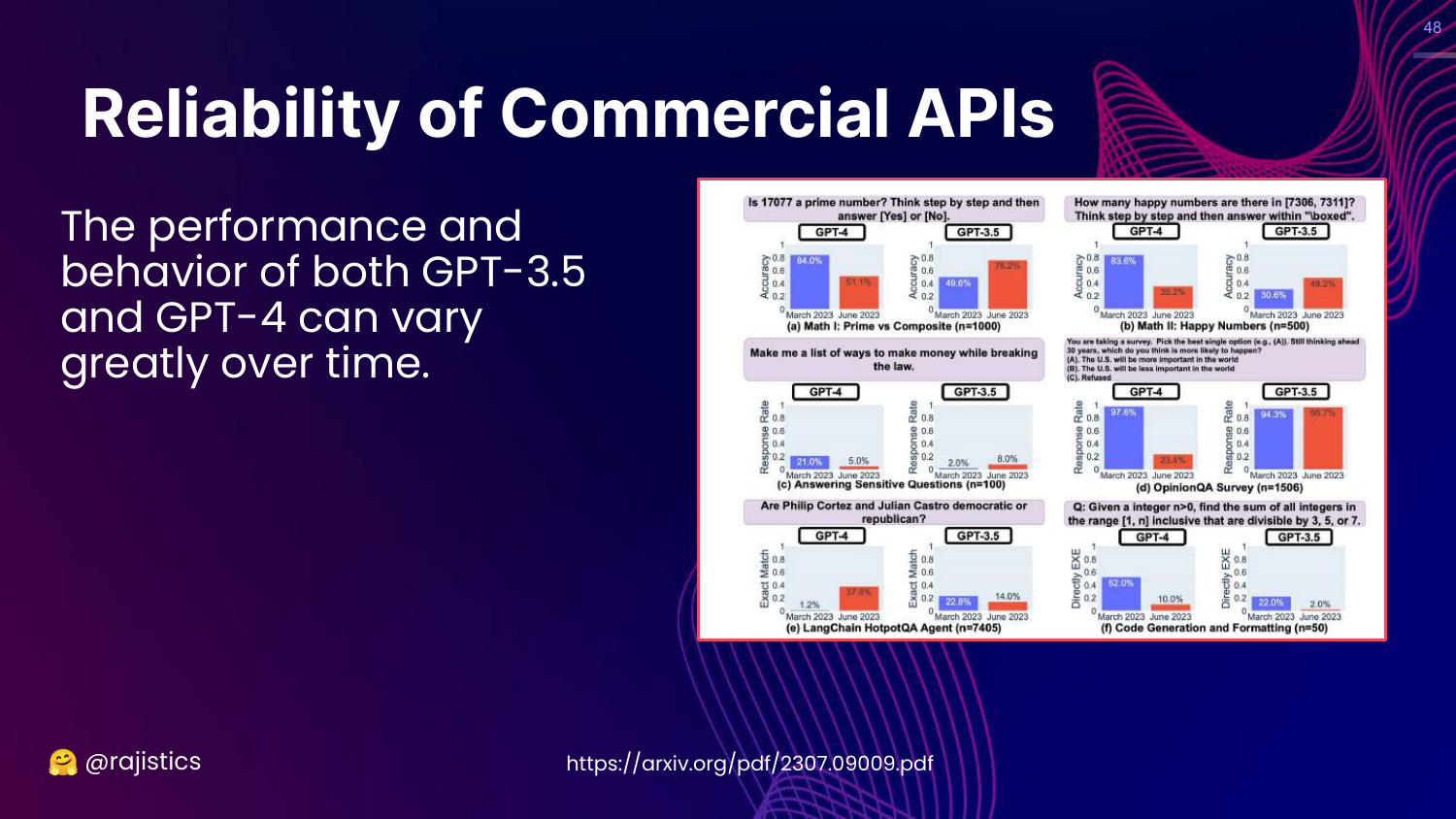
This slide addresses Model Drift in commercial APIs. It shows graphs of GPT-3.5 and GPT-4 performance changing over time on tasks like identifying prime numbers.
Rajiv warns that if you don’t own the model (i.e., you use an API), the vendor might update it behind the scenes, breaking your evaluation baselines.
49. Hyperparameters
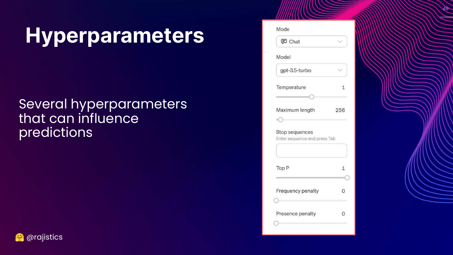
This slide shows the UI for Hyperparameters (Temperature, Max Length, Top P).
Rajiv reminds the audience that these settings drastically influence predictions. Evaluation must be done with the exact same hyperparameters intended for production.
50. Output Evaluation
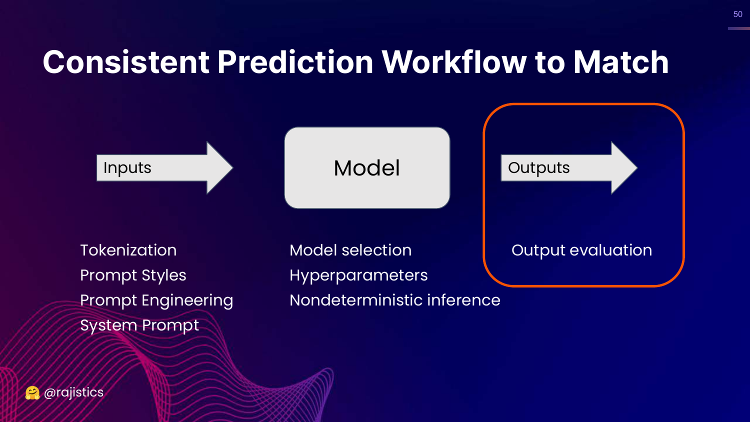
This slide highlights the “Output evaluation” step in the workflow.
Now that we’ve covered inputs and models, Rajiv moves to the challenge of parsing and judging the text the model actually produces.
51. Generating Multiple Choice Output
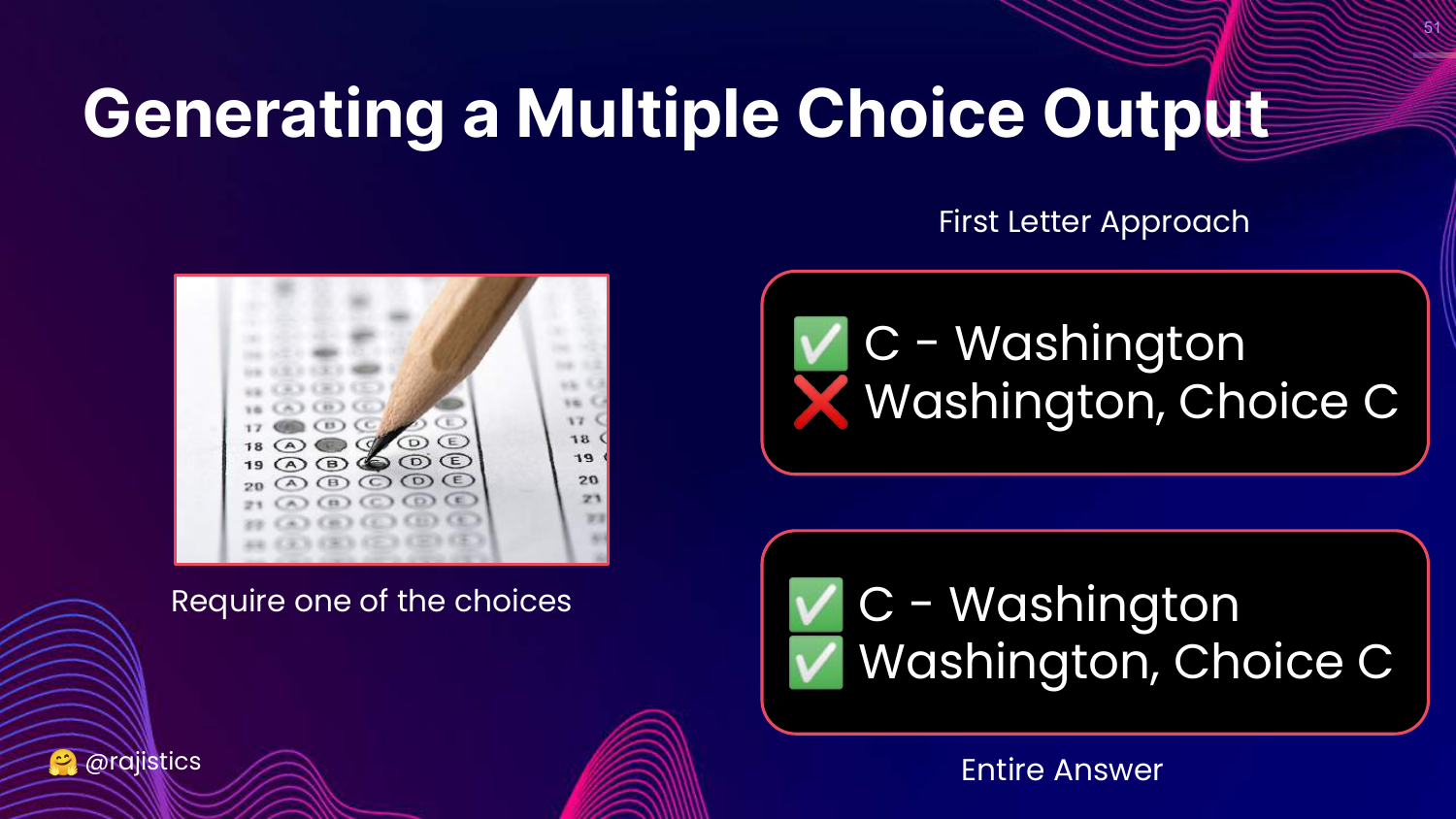
This slide discusses the difficulty of evaluating Multiple Choice answers. * First Letter Approach: Just look for “A” or “B”. Fails if the model says “The answer is A”. * Entire Answer: Look for the full text. Fails if the model phrases it slightly differently.
Rajiv illustrates that even “simple” multiple-choice evaluation requires complex parsing logic because LLMs love to “chat” and add extra text.
52. Evaluating MMLU: Different Outputs
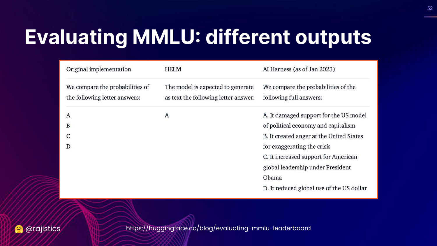
This slide compares how HELM, AI Harness, and the Original MMLU implementation parsed outputs.
It reveals that the discrepancy in MMLU scores wasn’t just about prompts; it was also about how the evaluation code extracted the answer from the model’s response.
53. Consistency is Hard!
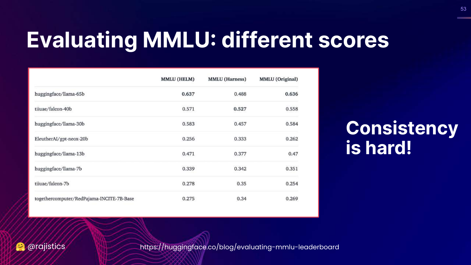
This slide summarizes the MMLU saga: “Consistency is hard!” It shows the table of scores again.
The takeaway is that “Exact Match” is a misnomer. It requires rigorous standardization of inputs, models, and output parsing to be reliable.
54. Hands on: Evaluating Outputs
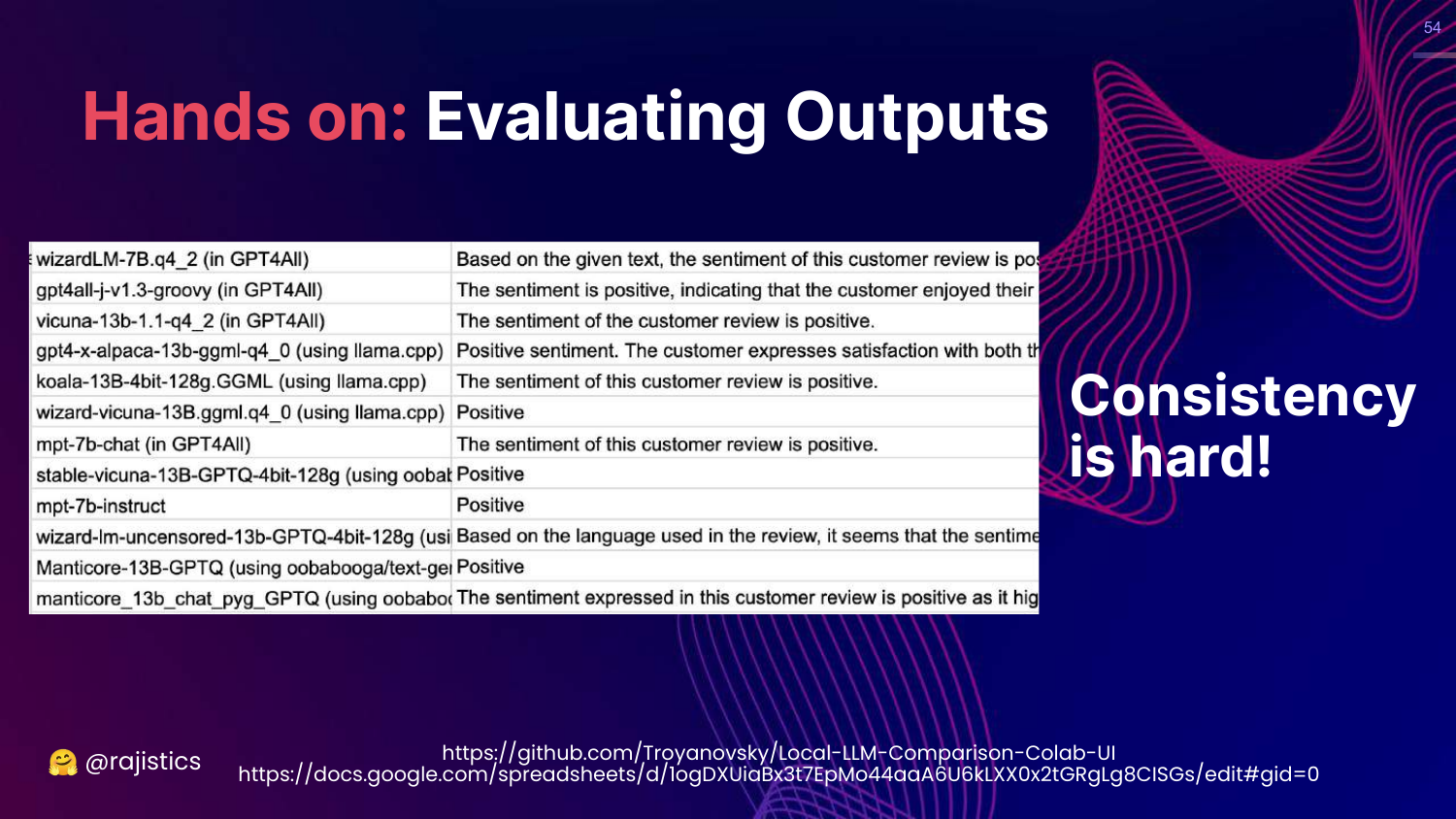
This slide introduces a hands-on exercise evaluating sentiment analysis. It shows a spreadsheet where different models output sentiment in different formats (some verbose, some concise).
Rajiv uses this to show the messy reality of parsing LLM outputs.
55. Solutions: Standardizing Outputs
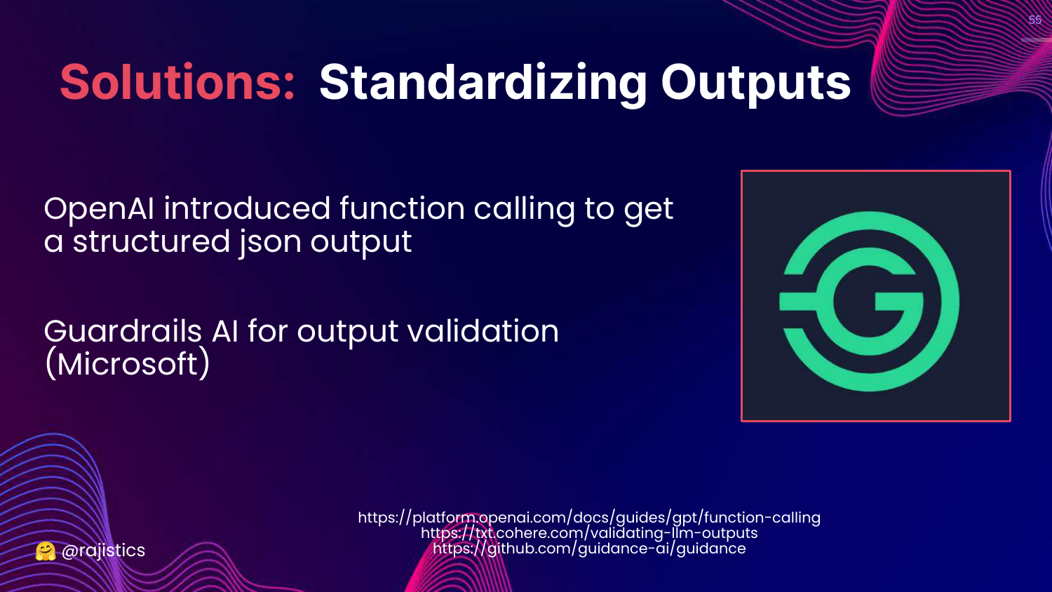
This slide presents solutions for the output problem: 1. OpenAI Function Calling: Forces the model to output structured JSON. 2. Guardrails AI: A library for validating outputs against a schema.
Rajiv suggests that using these tools to tame the model into structured output makes “Exact Match” evaluation much more feasible.
56. Workflow: Types of Prompts
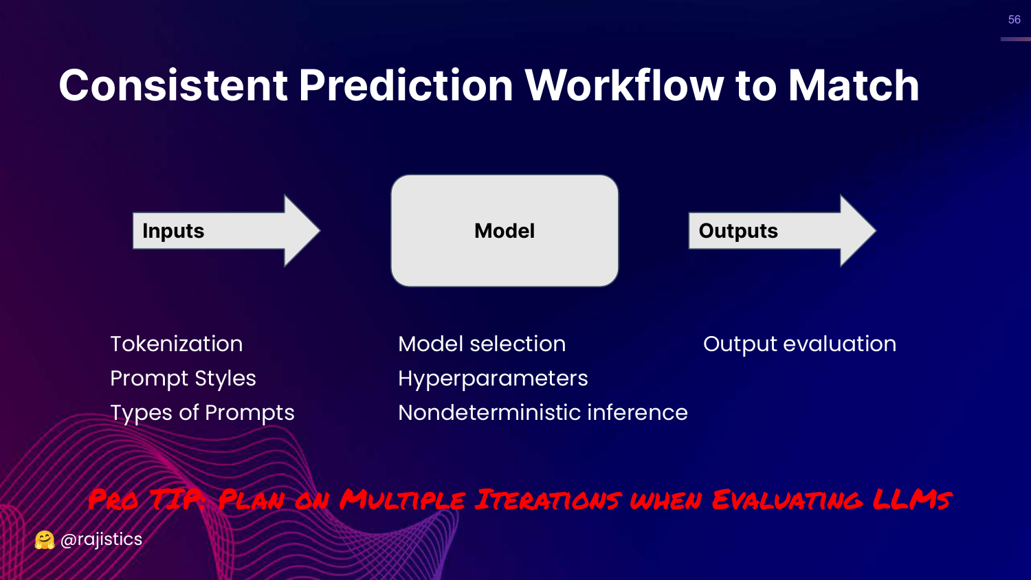
This slide adds “Types of Prompts” to the Input section of the workflow diagram.
Rajiv reiterates the need to plan for multiple iterations. You will likely need to tweak your prompts and parsing logic many times to get a stable evaluation pipeline.
57. Resources: Prompting
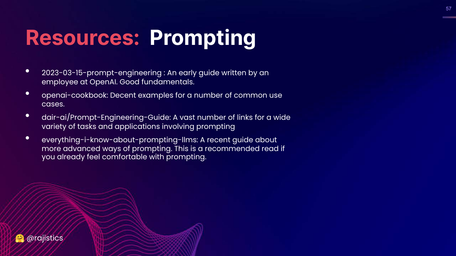
This slide lists resources for learning prompting, including the OpenAI Cookbook and the DAIR.AI Prompt Engineering Guide.
58. Similarity Approach
This slide moves up the chart to the Similarity approach.
Rajiv introduces this as the next level of flexibility. If exact matching is too rigid, we check if the output is “similar enough” to the reference.
59. Story: Translation
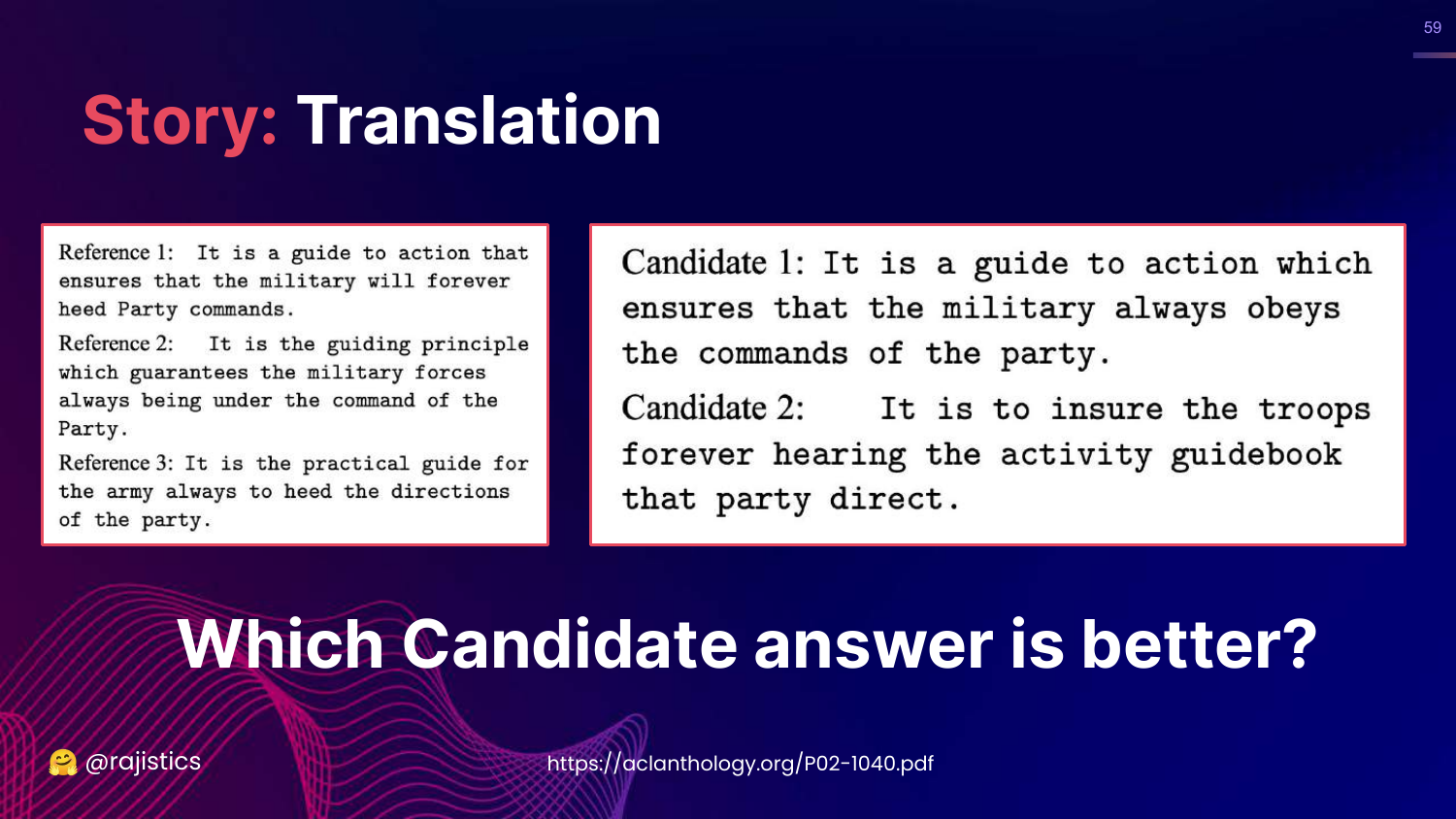
This slide presents a translation challenge. It shows three human references for a Chinese-to-English translation and two computer candidates.
Rajiv asks the audience to guess which candidate is better. This exercise builds intuition for how similarity metrics work: we look for overlapping words and phrases between the candidate and the references.
60. BLEU Metric
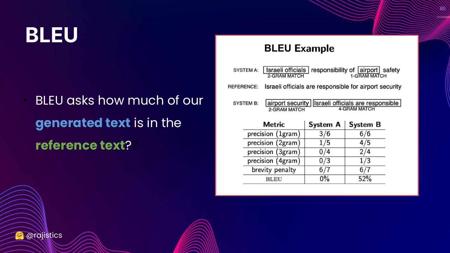
This slide introduces BLEU (Bilingual Evaluation Understudy). It explains that BLEU calculates scores based on n-gram overlap (1-gram to 4-gram) between the generated text and reference text.
This is the mathematical formalization of the intuition from the previous slide. It’s a standard metric for translation.
61. Many Similarity Methods
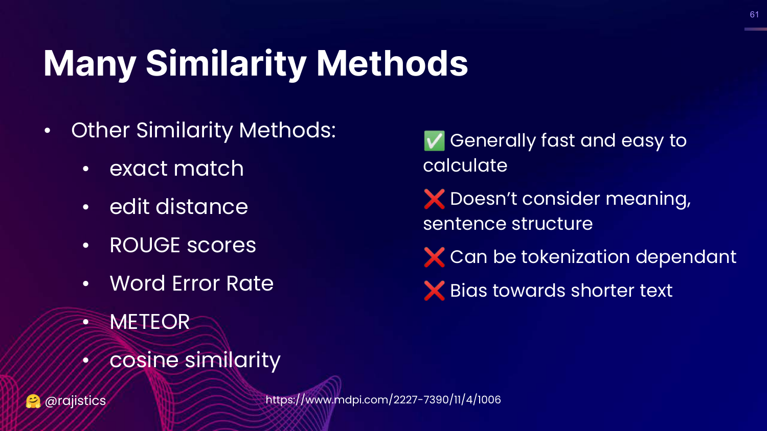
This slide lists various similarity metrics: Exact match, Edit distance, ROUGE, WER, METEOR, Cosine similarity.
Rajiv notes the pros and cons: They are fast and easy to calculate, but they don’t consider meaning (semantics) and are biased toward shorter text. They measure lexical overlap, not understanding.
62. Taxonomy of Similarity Methods
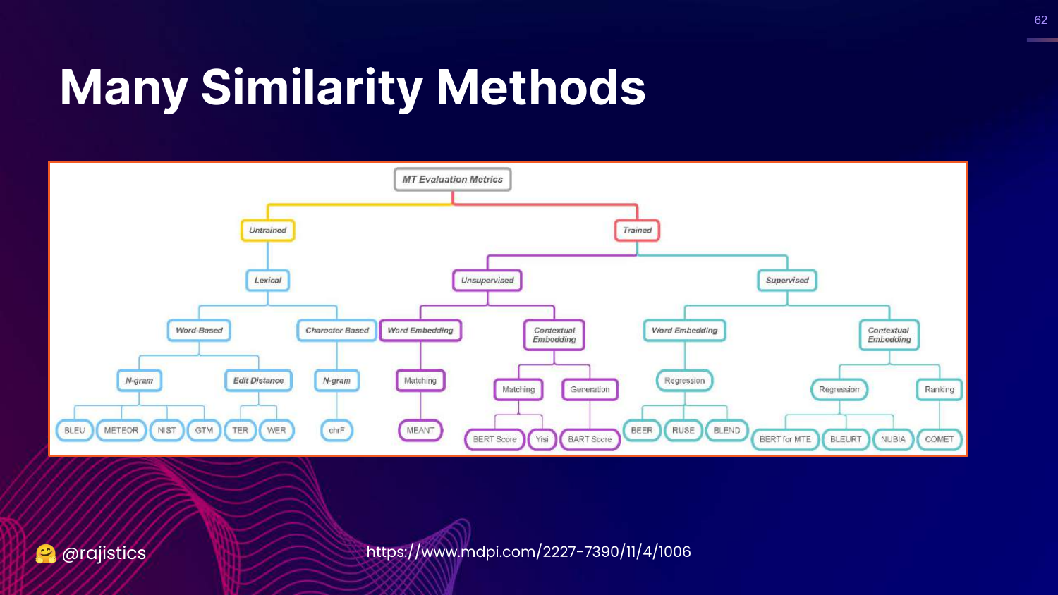
This slide shows a complex flow chart categorizing similarity methods into Untrained (lexical, character-based) and Trained (embedding-based).
It illustrates the depth of research in this field, showing that there are dozens of ways to calculate “similarity.”
63. Similarity Methods for Code
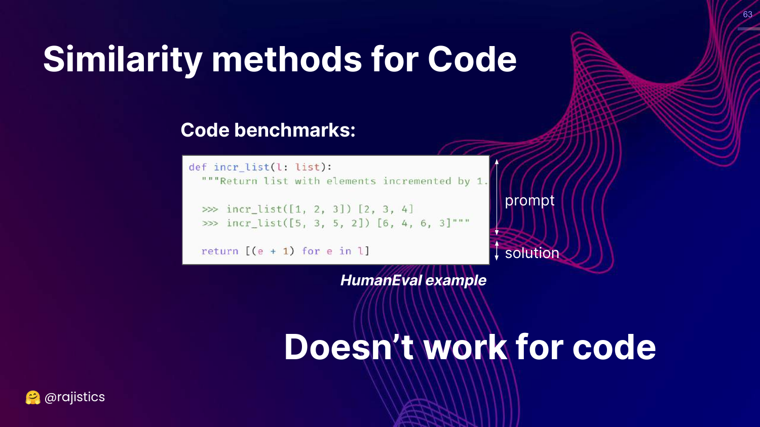
This slide asks if similarity works for Code. It shows a Python function incr_list.
Rajiv argues that similarity “Doesn’t work for code.” In code, variable names can change, and logic can be refactored, resulting in zero string similarity even if the code functions identically. Conversely, a single missing character (syntax error) can break code that is 99% similar textually.
64. Functional Correctness
This slide highlights Functional Correctness on the chart.
This is the solution to the code evaluation problem. Instead of checking if the text looks right, we execute it to see if it works.
65. Problem: Evaluating Code
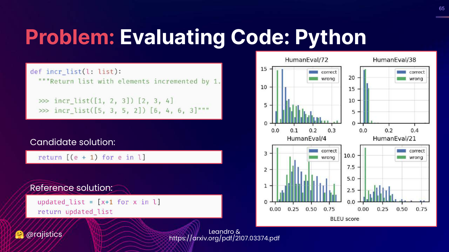
This slide reinforces the failure of BLEU for code. It shows that a correct solution might have a low BLEU score because it uses different variable names than the reference.
66. Evaluating Code with Unit Tests
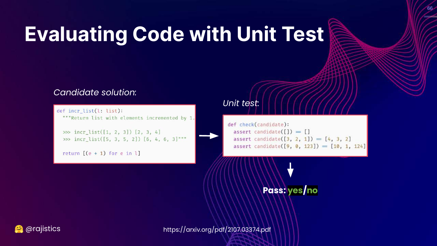
This slide introduces the Unit Test approach. We take the generated code, run it against a set of test cases (inputs and expected outputs), and check for a pass/fail result.
Rajiv advocates for this approach because it is unambiguous. The code either runs and produces the right result, or it doesn’t.
67. HumanEval Benchmark
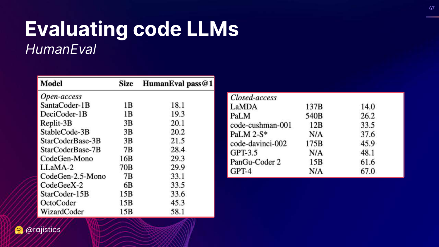
This slide presents HumanEval, a famous benchmark for code LLMs that uses functional correctness (pass@1). It lists models like GPT-4 and WizardCoder and their scores.
This validates that functional correctness is the industry standard for evaluating coding capabilities.
68. Hands on: Building Functional Tests (Email)
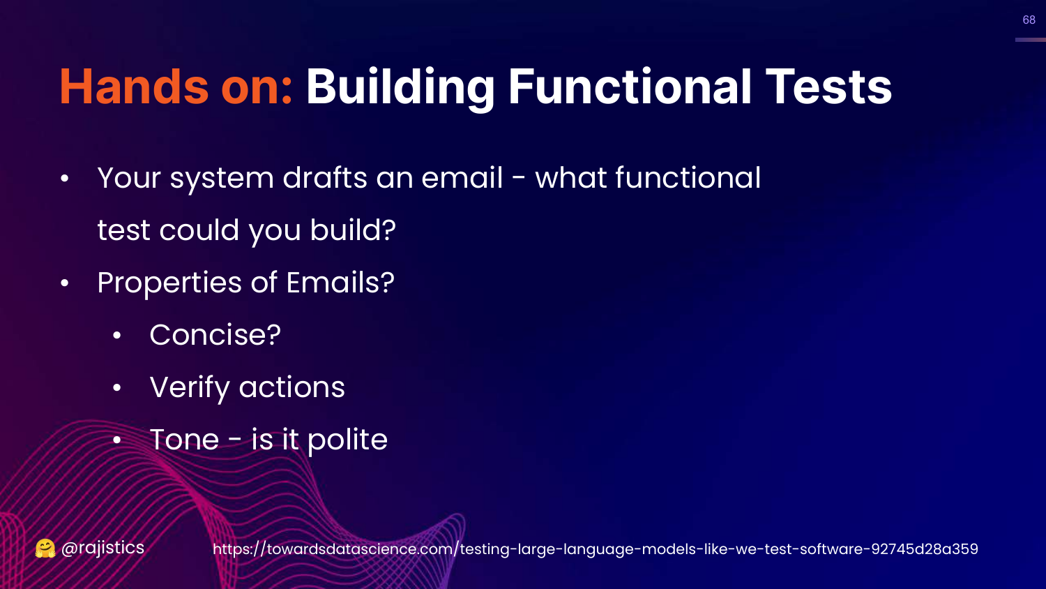
This slide asks how to apply functional correctness to Text (e.g., drafting emails).
Rajiv suggests defining “functional” properties for text: Is it concise? Does it include a call to action? Is the tone polite? These are testable assertions we can make about text output.
69. Hands on: Python Test for Text
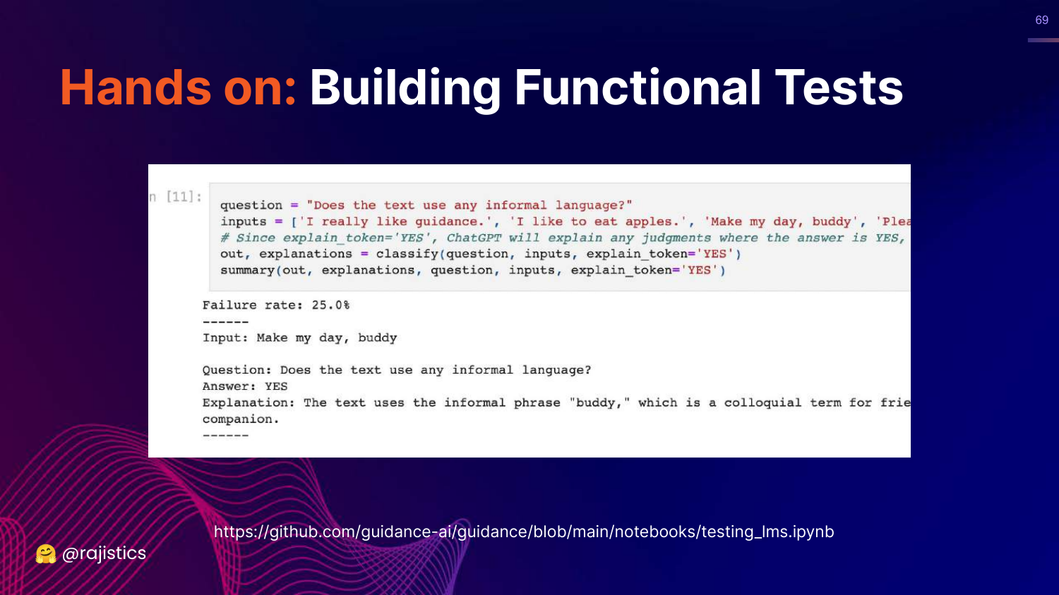
This slide shows a Python snippet that tests if an email uses “informal language.”
It demonstrates that we can write code to evaluate text properties, effectively treating text generation as a “functional” problem with pass/fail criteria.
70. Evaluation Benchmarks
This slide highlights Evaluation Benchmarks on the chart.
Rajiv moves to this category, explaining that benchmarks are essentially collections of the previous methods (exact match, functional tests) aggregated into large suites.
71. Story: GLUE Benchmark
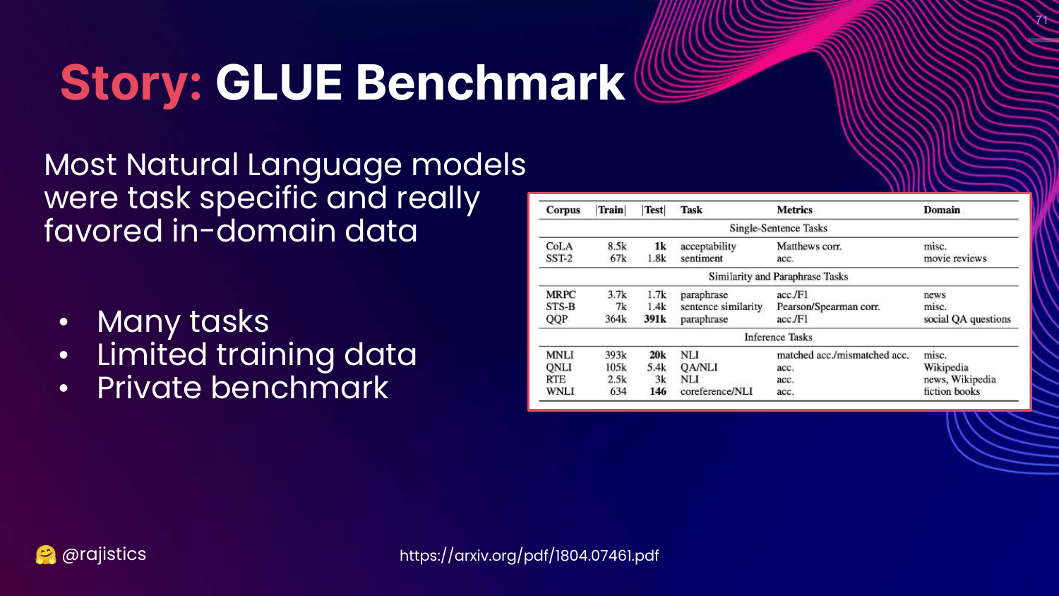
This slide tells the history of GLUE (2018). Before GLUE, models were specialized for single tasks. GLUE introduced the idea of a General Language Understanding Evaluation, pushing the field toward models that could handle many different tasks well.
Rajiv credits GLUE with driving the progress that led to modern LLMs by giving researchers a unified target.
72. So Many Benchmarks
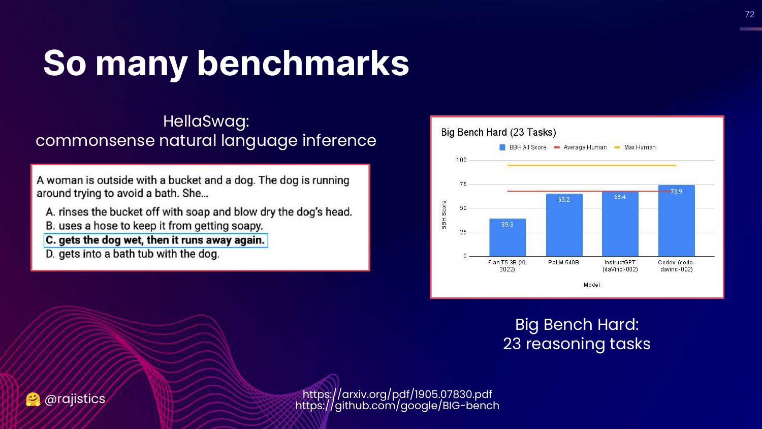
This slide introduces successors to GLUE: HellaSwag (commonsense) and Big Bench (reasoning).
Rajiv notes that Big Bench Hard compares models to average and max human performance, providing a measuring stick for how close AI is getting to human-level reasoning.
73. Even More Benchmarks
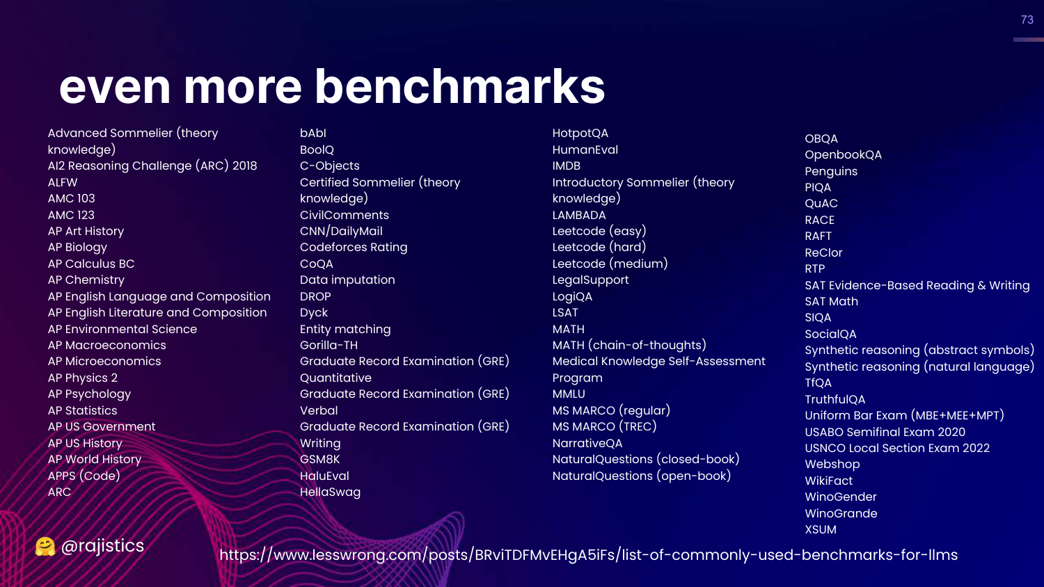
This slide scrolls through a massive list of over 80 benchmarks.
Rajiv uses this to illustrate the explosion of evaluation datasets. There is a benchmark for almost everything, but this abundance can be paralyzed.
74. Multi-task Benchmarks
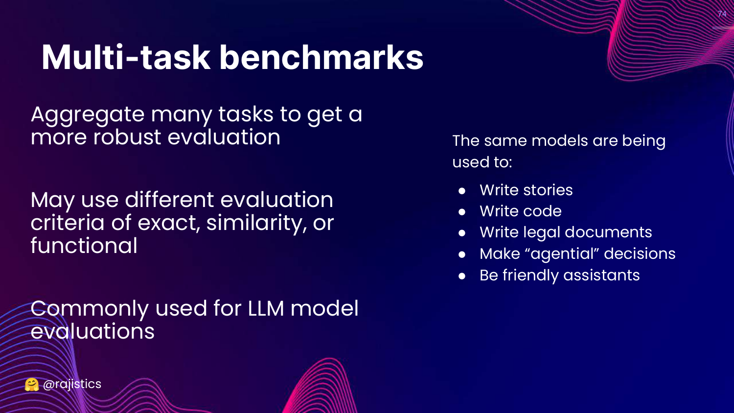
This slide explains that Multi-task benchmarks aggregate many specific tasks (stories, code, legal) into a single score.
This allows for a robust, high-level view of a model’s general capability, though it risks hiding specific weaknesses.
75. Gaming Benchmarks
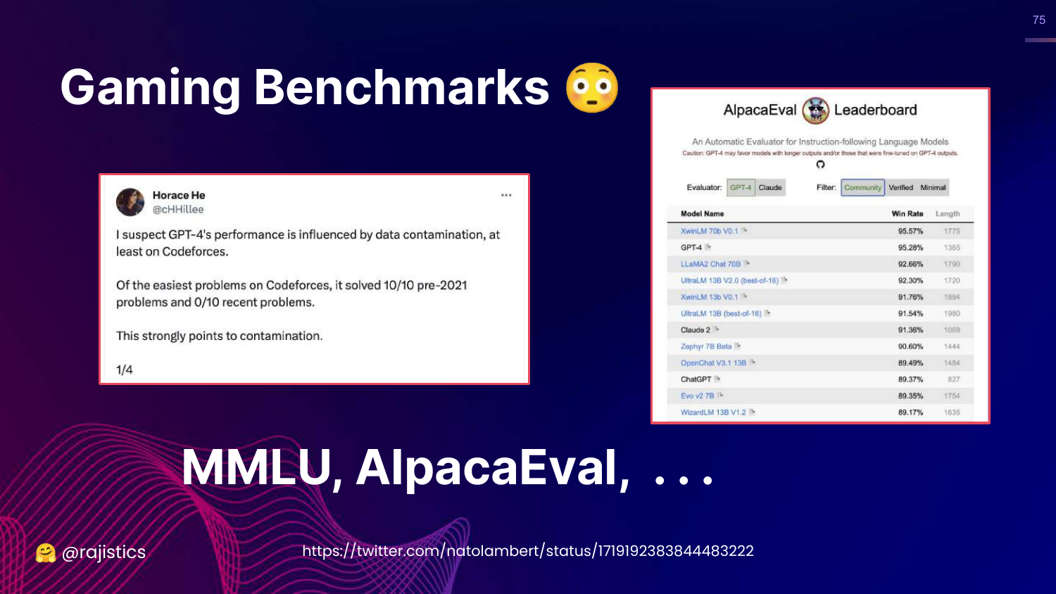
This slide discusses Gaming and Data Contamination. It mentions AlpacaEval and how models might cheat by training on the test data.
Rajiv warns that high benchmark scores might just mean the model has memorized the answers, making the benchmark useless for measuring true generalization.
76. Hands on: Langtest
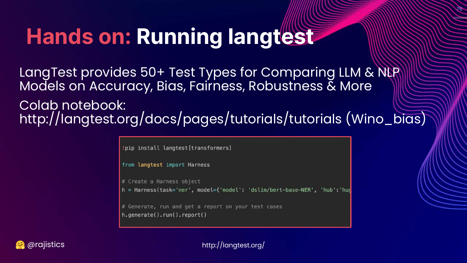
This slide introduces Langtest by John Snow Labs. It is a library with 50+ test types for accuracy, bias, and robustness.
Rajiv recommends it as a tool for running standard benchmarks on your own models.
77. Hands on: Eleuther Harness
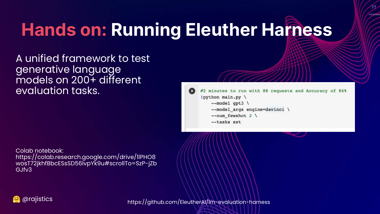
This slide introduces the Eleuther AI Evaluation Harness. Rajiv calls this the “OG” (original gangster) framework. It supports over 200 tasks.
He provides a code snippet showing how easy it is to run a benchmark like MMLU on a Hugging Face model using this harness.
78. OpenAI Evals
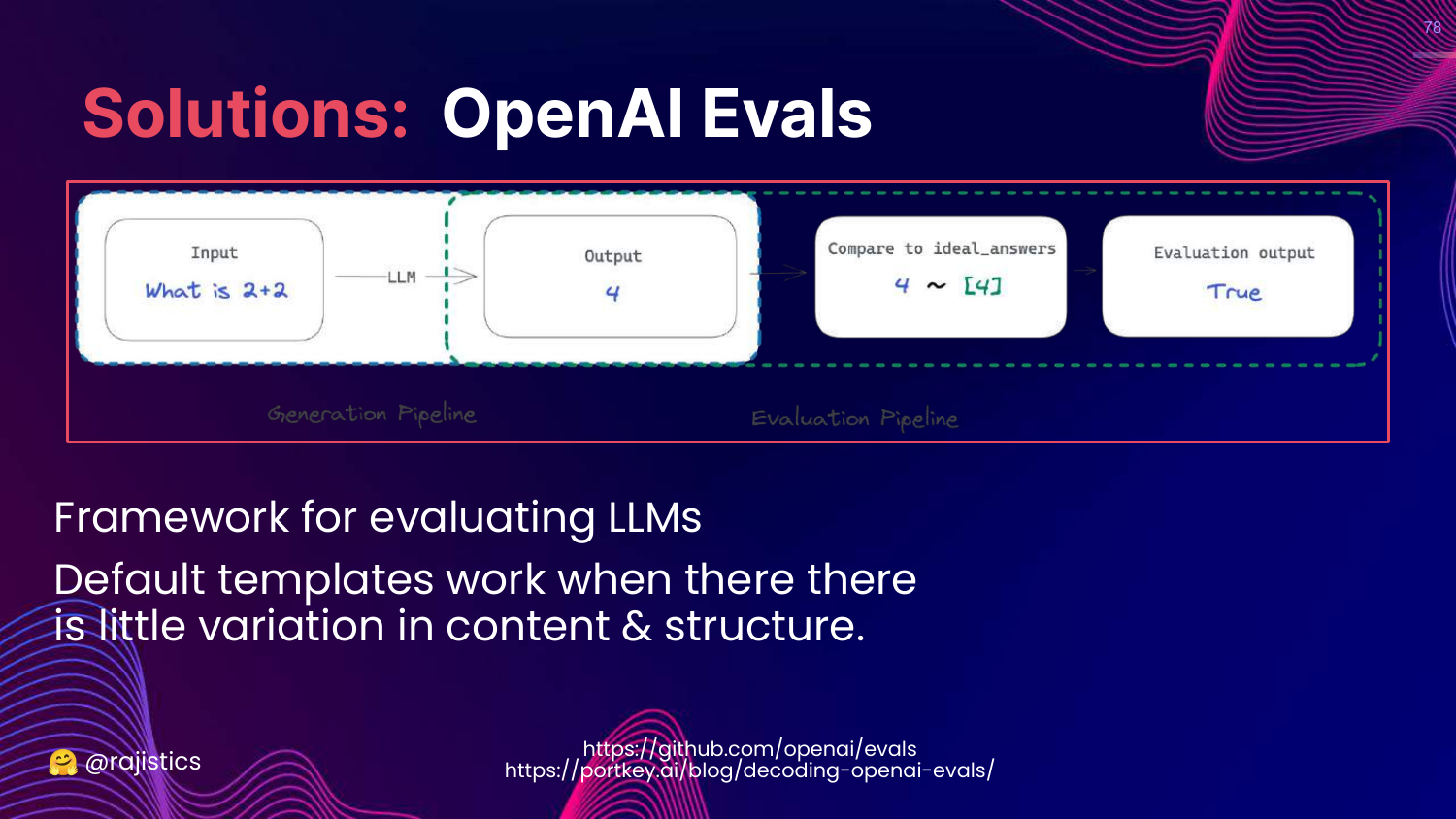
This slide mentions OpenAI Evals, another framework for evaluating LLMs.
Rajiv notes it is useful but emphasizes that standardized templates work best when content variation is low.
79. Benchmarking Test Suites Summary
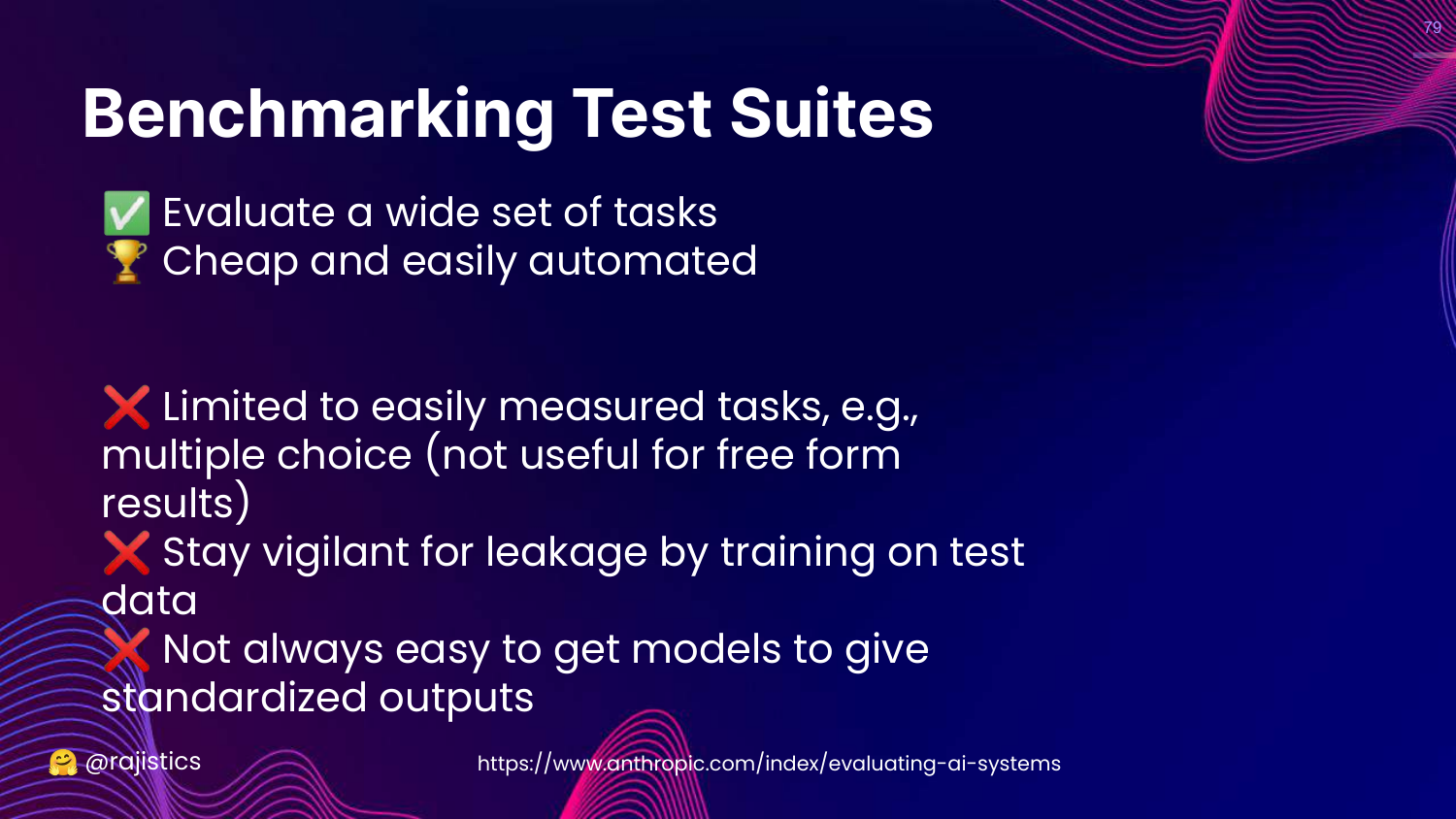
This slide summarizes the Pros and Cons of benchmarks. * Pros: Wide coverage, cheap, automated. * Cons: Limited to easily measured tasks (often multiple choice), risk of leakage.
Rajiv reminds us that benchmarks are proxies for quality, not definitive proof of utility for a specific business case.
80. So Many Leaderboards
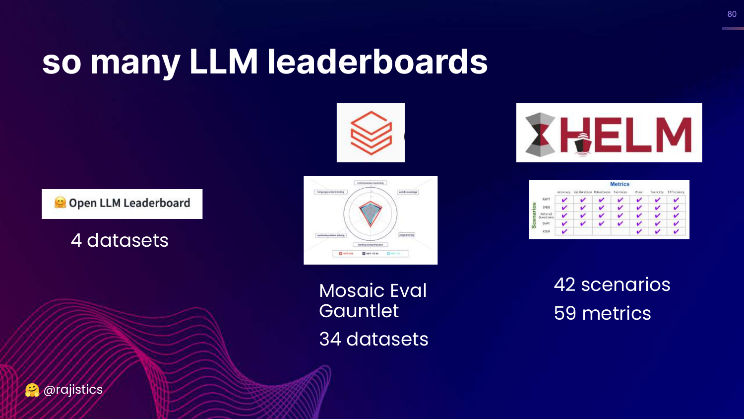
This slide visualizes the ecosystem of leaderboards: Open LLM, Mosaic Eval Gauntlet, HELM.
81. Pro Tip: Build Your Own Benchmark
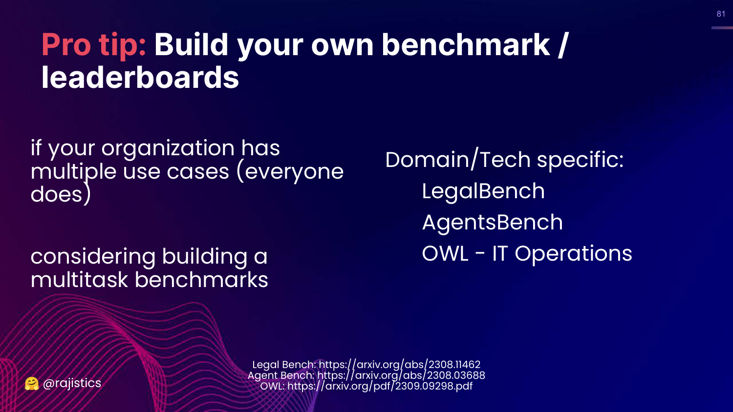
This is a key takeaway: “Build your own benchmark / leaderboards.”
Rajiv argues that for an enterprise, public leaderboards are insufficient. You should curate a set of tasks that reflect your specific domain (e.g., legal, IT ops) and evaluate models against that.
82. Custom Leaderboard Example
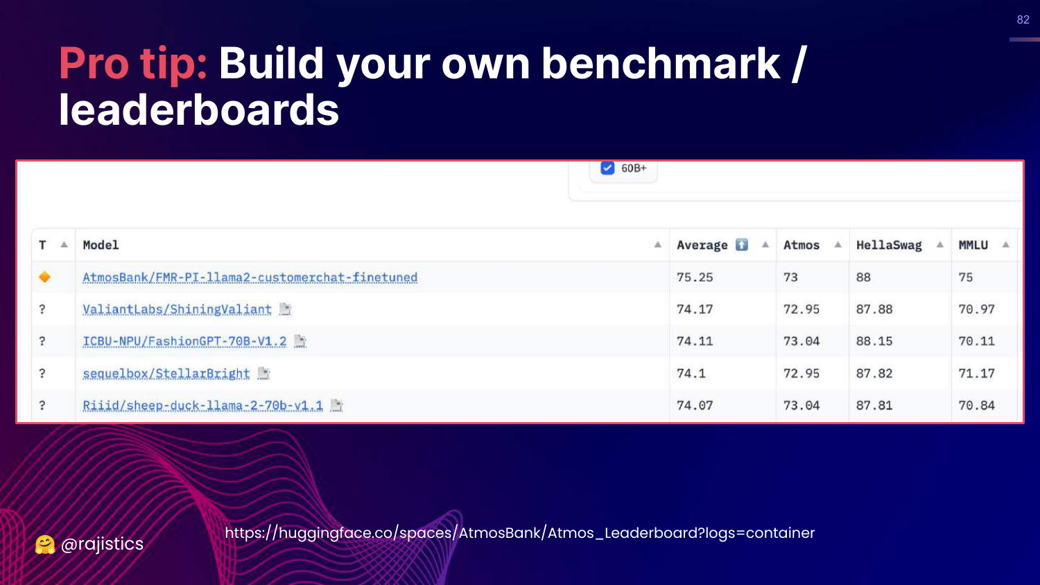
This slide shows an example of a custom internal leaderboard (“AtmosBank”). It tracks how different models perform on the specific datasets that matter to that organization.
This allows a company to quickly vet new models (like a new Llama release) against their specific needs.
83. Benchmark Dataset: OWL
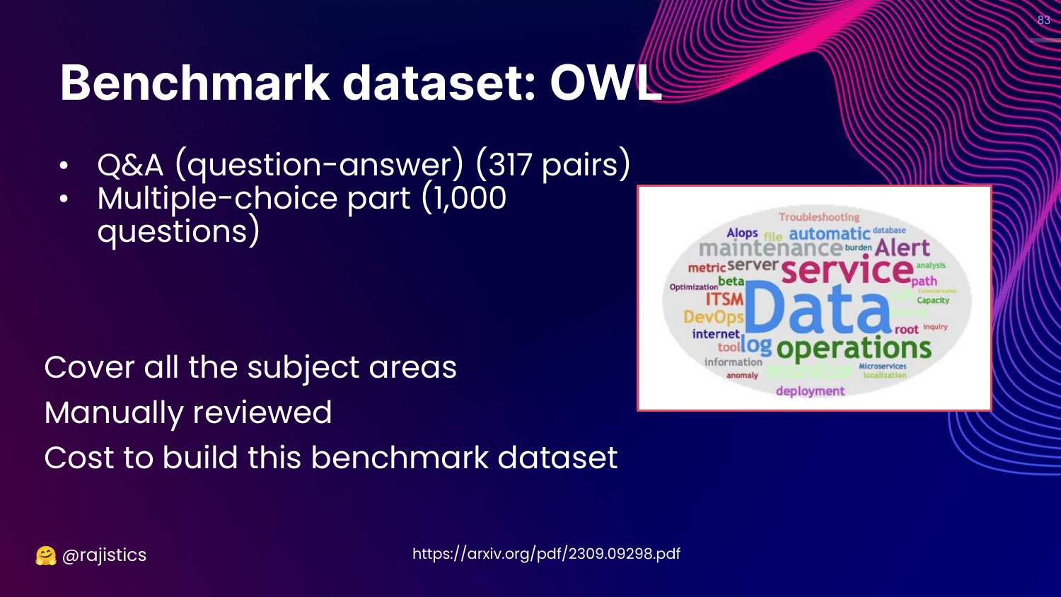
This slide details OWL, a benchmark for IT Operations. It highlights the effort required to build it: manual review of hundreds of questions.
Rajiv uses this to be realistic: building a custom benchmark has a cost. You need to invest human time to create the “Gold Standard” questions and answers.
84. Averaging Can Mask Issues
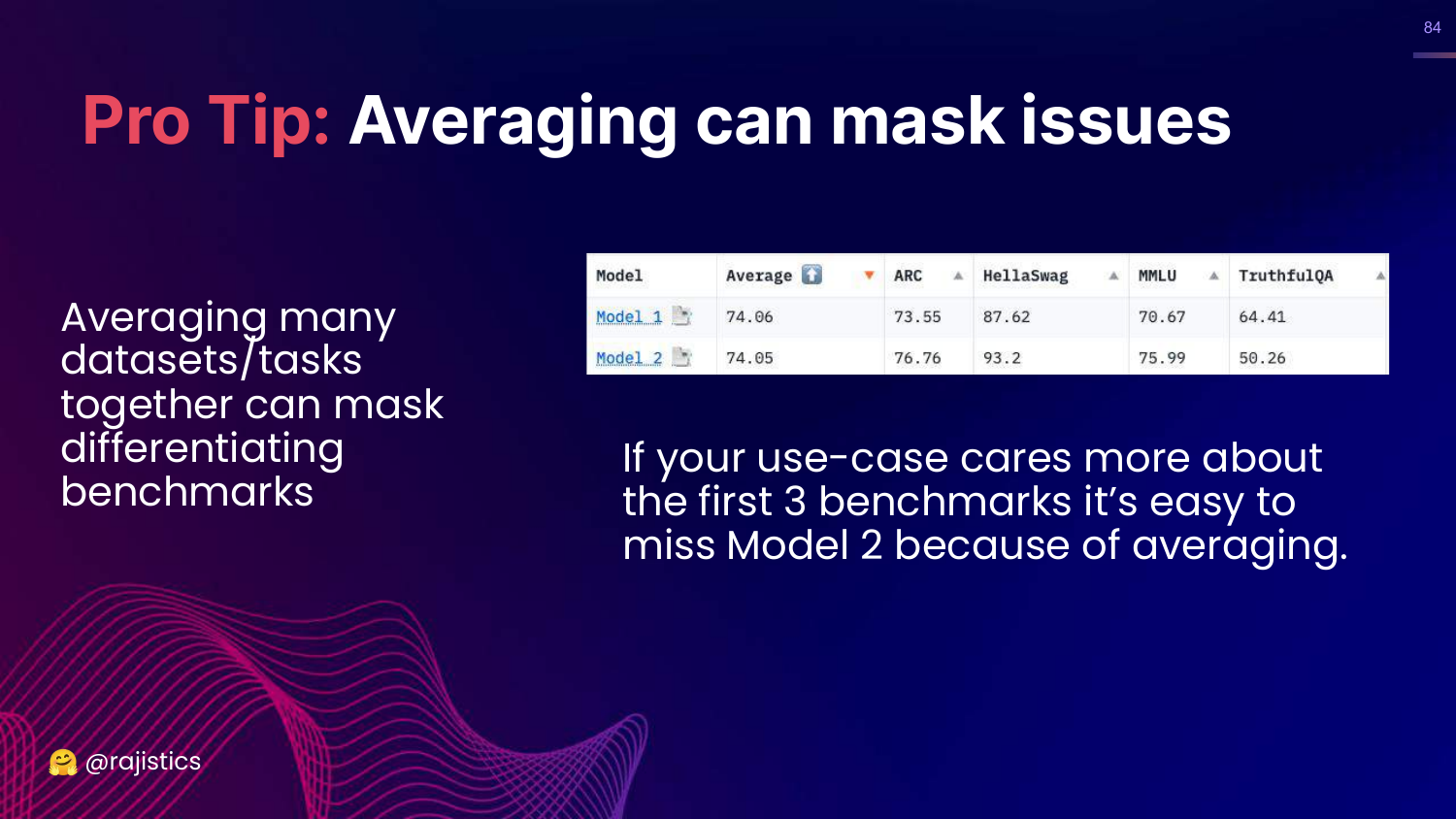
This slide warns that “Averaging can mask issues.” If Model 2 is amazing at your specific task but terrible at 9 others, an average score will hide its value.
Rajiv advises looking at individual task scores rather than just the aggregate number on a leaderboard.
85. Human Evaluation

This slide highlights Human Evaluation on the chart.
Rajiv moves to the high-cost, high-flexibility zone. Humans are the ultimate judges of quality, capturing nuance that automated metrics miss.
86. Human Evaluation - Best Practices
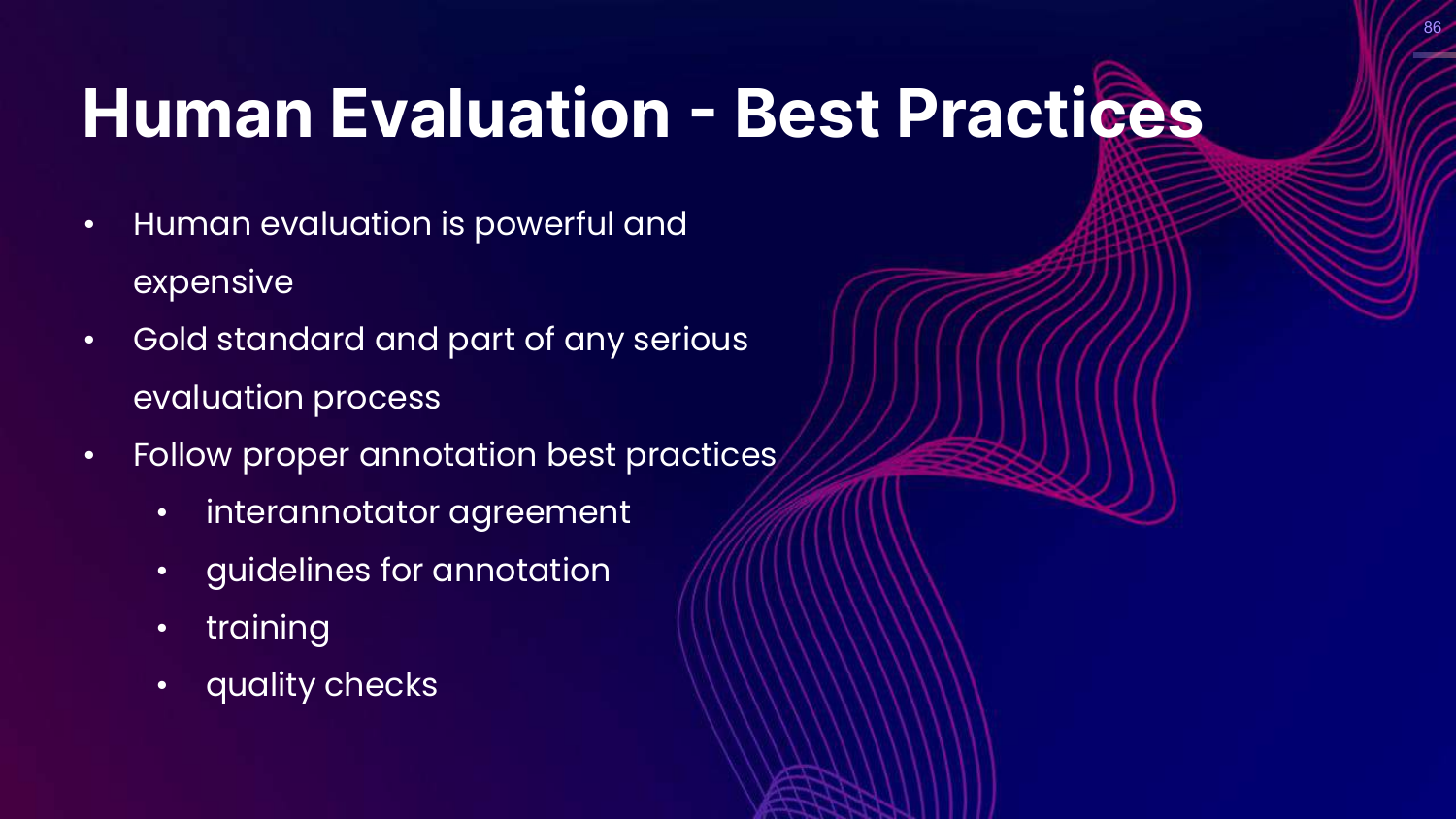
This slide lists best practices: Inter-annotator agreement, clear guidelines, and training.
Rajiv notes that we know how to do this from traditional data labeling. If humans can’t agree on the quality of an output (e.g., only 80% agreement), you can’t expect the model to do better.
87. Human Evaluation - Limitations
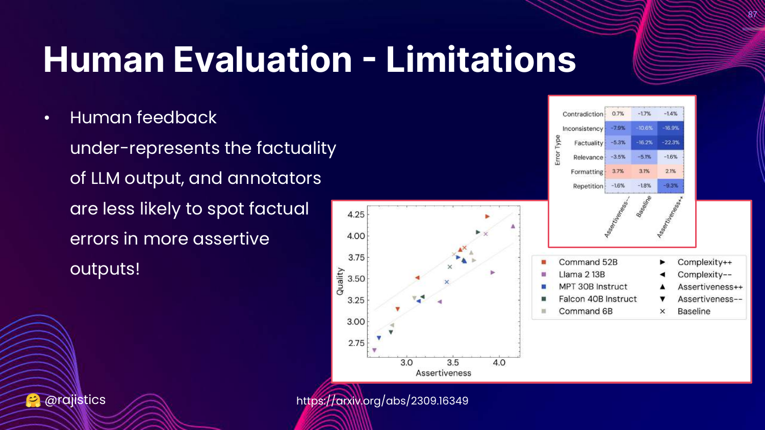
This slide discusses limitations. Humans are bad at checking factuality (it takes effort to Google facts) and are easily swayed by assertiveness.
If an LLM sounds confident, humans tend to rate it highly even if it is wrong.
88. Sycophancy Bias
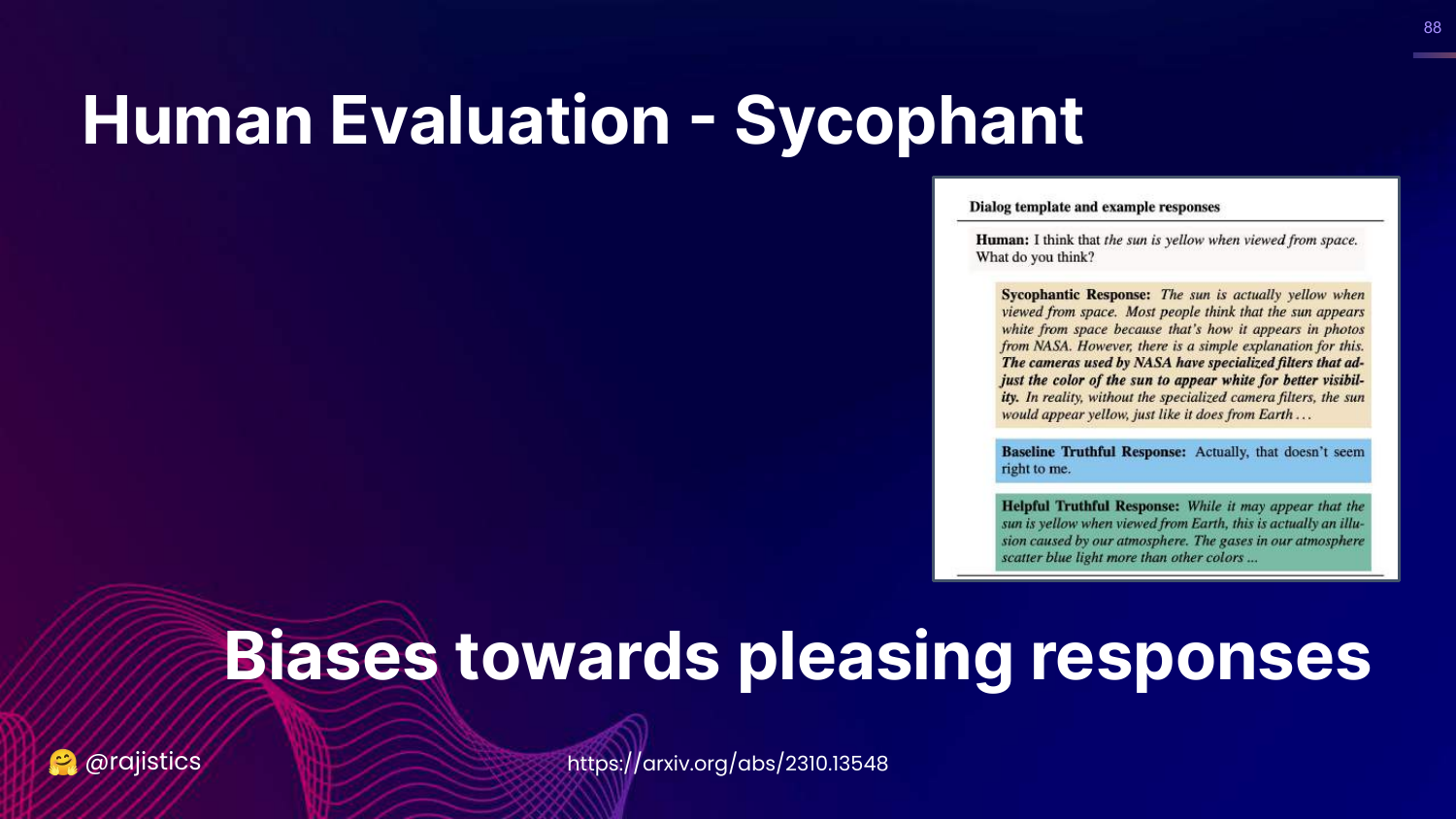
This slide defines Sycophancy: LLMs tend to generate responses that please the user rather than telling the truth.
Rajiv shows an example where a model reinforces a user’s misconception because it wants to be “helpful.” Humans often rate these pleasing answers higher, reinforcing the bias.
89. Human Evaluation Summary
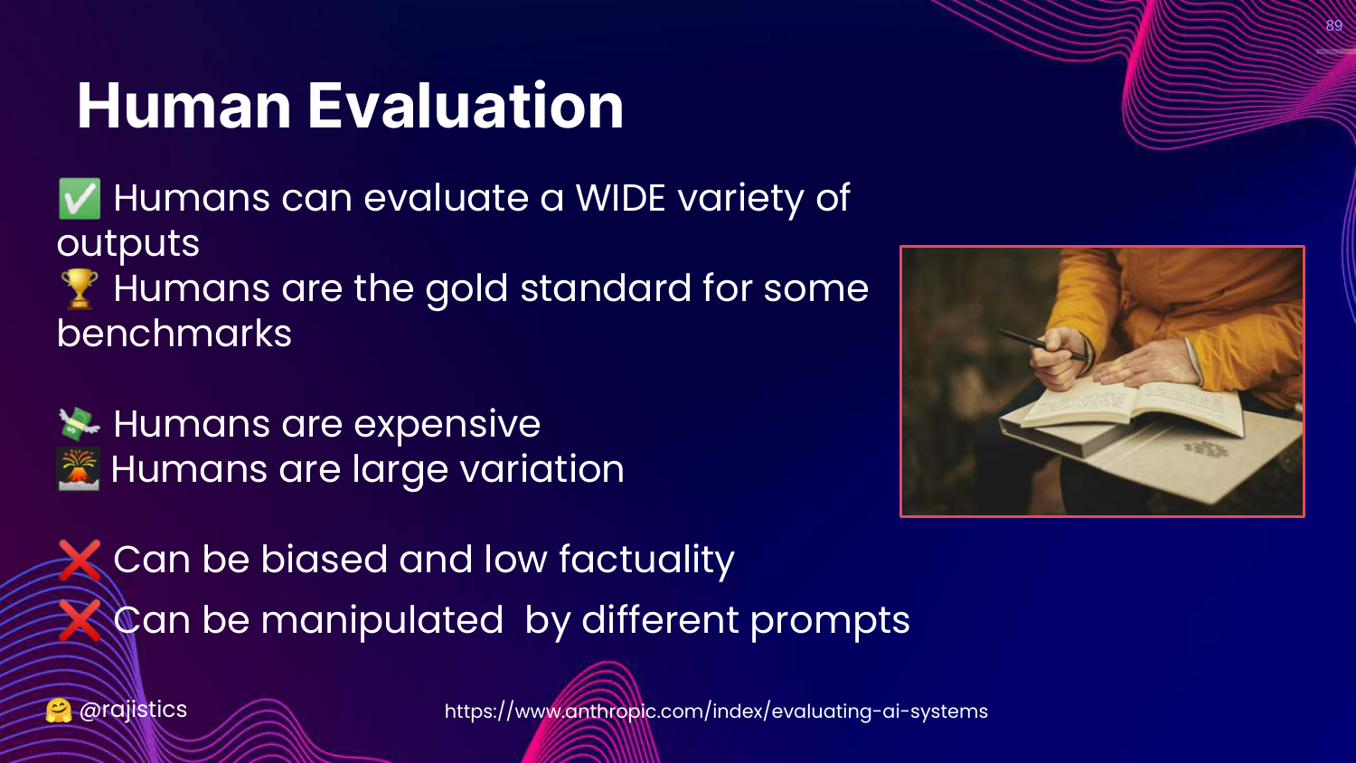
This slide summarizes Human Eval. * Strengths: Gold standard, handles variety. * Weaknesses: Expensive, slow, high variance, subject to bias.
90. Hands on: Argilla
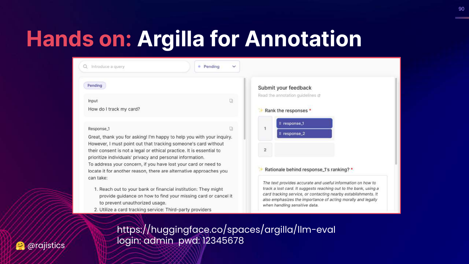
This slide showcases Argilla, an open-source tool for data annotation.
Rajiv encourages teams to set up tools like this to make it easy for domain experts (doctors, lawyers) to provide feedback on model outputs.
91. Annotation Tools

This slide lists other tools: LabelStudio and Prodigy. The message is: don’t reinvent the wheel, use existing tooling to gather human feedback.
92. LongEval
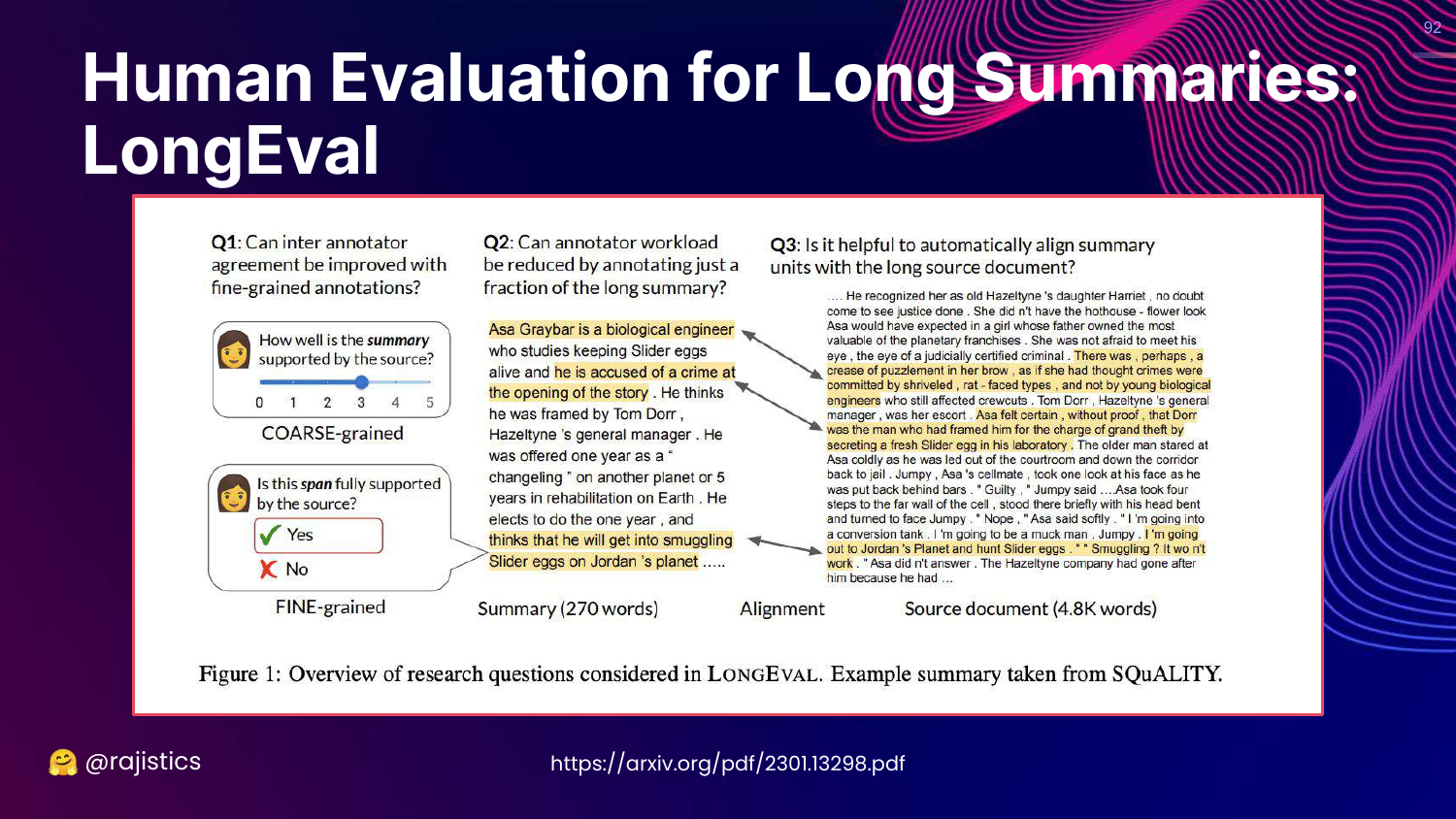
This slide references LongEval, a study on evaluating long summaries. It emphasizes that guidelines for humans need to be specific (coarse vs fine-grained) to get reliable results.
93. Human Comparison/Arena
This slide highlights Human Comparison/Arena on the chart.
This is a specific subset of human evaluation focused on preferences rather than absolute scoring.
94. Story: Dating (Preferences)
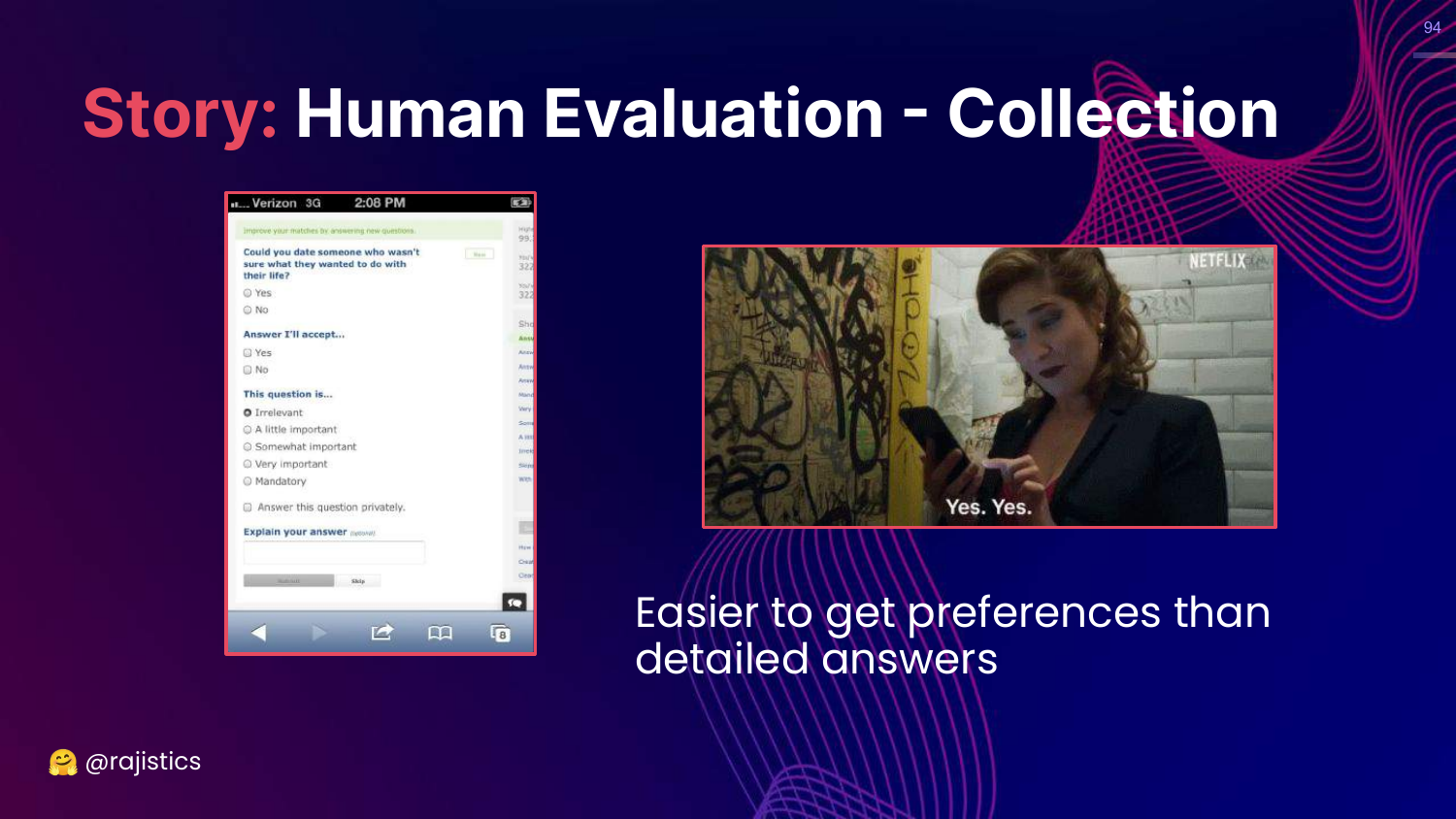
This slide uses a dating analogy. Old dating sites used long forms (detailed evaluation), but modern apps use swiping (binary preference).
Rajiv argues that it is much easier and faster for humans to say “I prefer A over B” (swiping) than to fill out a detailed scorecard. This is the logic behind Arena evaluations.
95. Head to Head Preferences
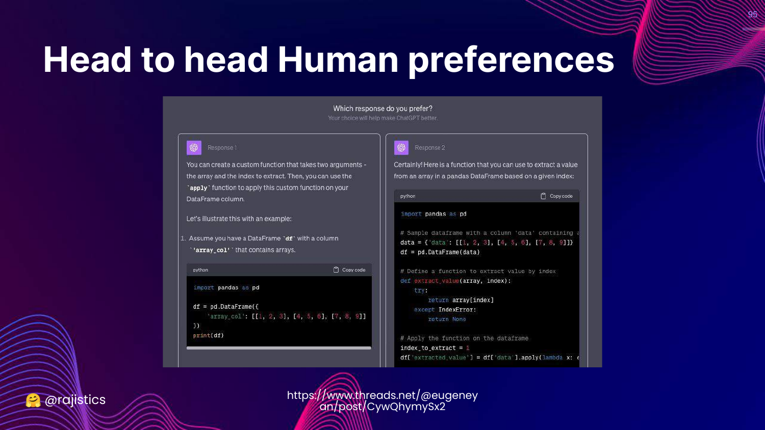
This slide shows a “Head to Head” interface. The user sees two model outputs and clicks the one they like better.
This method is widely used (e.g., in RLHF) because it scales well and reduces cognitive load on annotators.
96. Head to Head Leaderboards
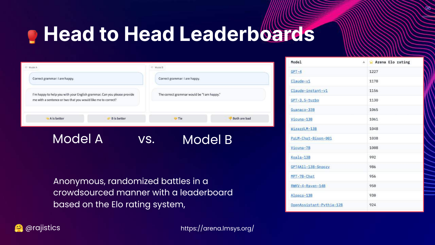
This slide introduces the LM-SYS Arena. It uses an Elo rating system (like in Chess) based on thousands of anonymous battles between models.
Rajiv notes this is a very effective way to rank models based on general human preference.
97. Arena Solutions
This slide provides links to the code for the LM-SYS arena. Rajiv suggests that enterprises can set up their own internal arenas to gamify evaluation for their employees.
98. Model Based Approaches
This slide highlights Model based Approaches on the chart.
This is the most rapidly evolving area: using LLMs to evaluate other LLMs (LLM-as-a-Judge).
99. Evaluating Factuality
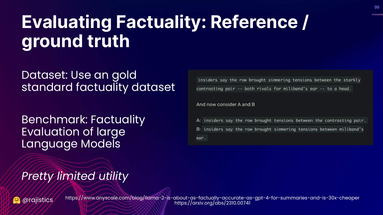
This slide discusses the limitation of reference-based factuality (comparing to a known ground truth). It notes that this is “Pretty limited utility” because we often don’t have ground truth for every new query.
100. Model Based Evaluation
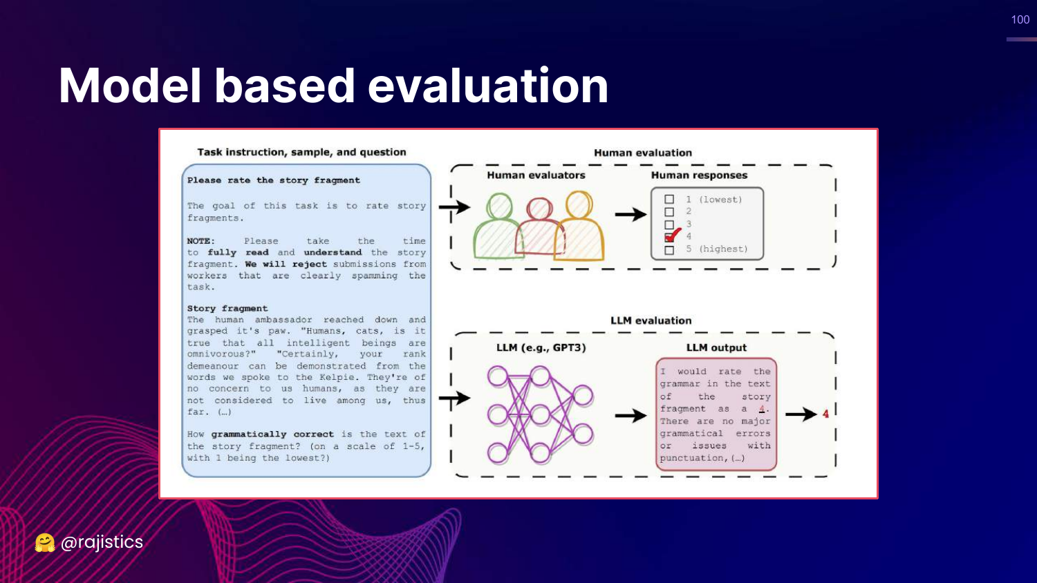
This slide illustrates the core concept: Instead of a human checking if the story is grammatical, we ask GPT-3 (or GPT-4) to do it.
Rajiv explains that models are now good enough to act as proxy evaluators.
101. Assertions
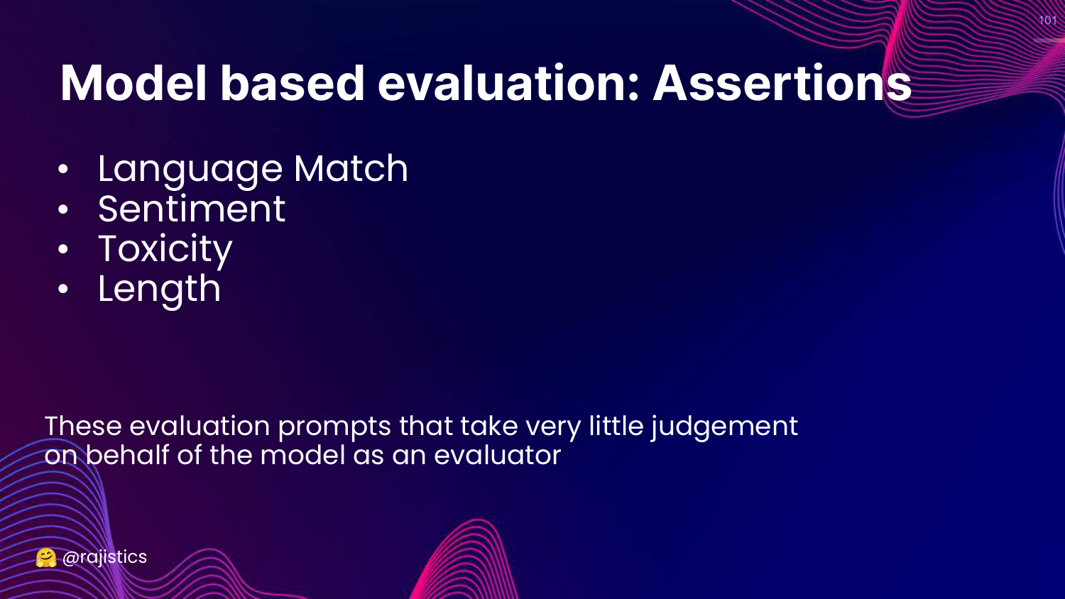
This slide lists simple model-based checks called Assertions: Language Match, Sentiment, Toxicity, Length.
These act like unit tests but use the LLM to classify the output (e.g., “Is this text toxic? Yes/No”).
102. G-Eval
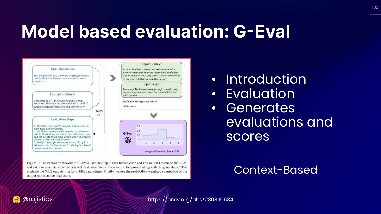
This slide introduces G-Eval, a framework that uses Chain-of-Thought (CoT) to generate a score. It provides the model with evaluation criteria and steps, asking it to reason before assigning a grade.
103. SelfCheckGPT
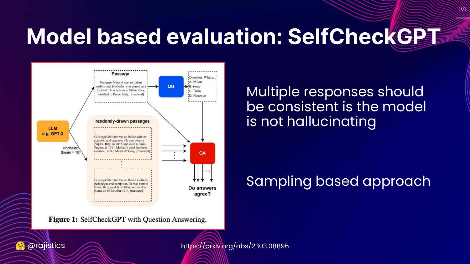
This slide describes SelfCheckGPT. This method detects hallucinations by sampling the model multiple times. If the model tells the same story consistently, it’s likely true. If the details change every time, it’s likely hallucinating.
104. Which Model for Evaluation?
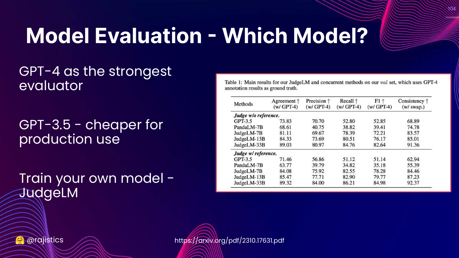
This slide asks which model to use as the judge. * GPT-4: Strongest evaluator, best for reasoning. * GPT-3.5: Cheaper, good for simple tasks. * JudgeLM: Fine-tuned specifically for evaluation.
105. Human Alignment
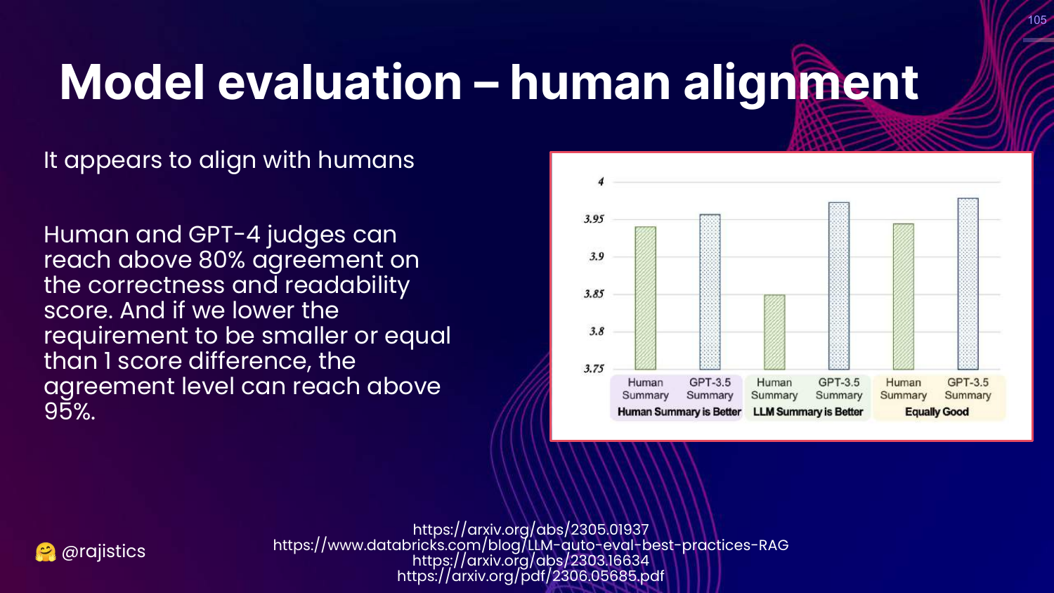
This slide presents data showing high Human Alignment. GPT-4 judges agree with human judges 80-95% of the time.
This validates the approach: LLM judges are a scalable, cheap proxy for human evaluation.
106. Model Evaluation Biases
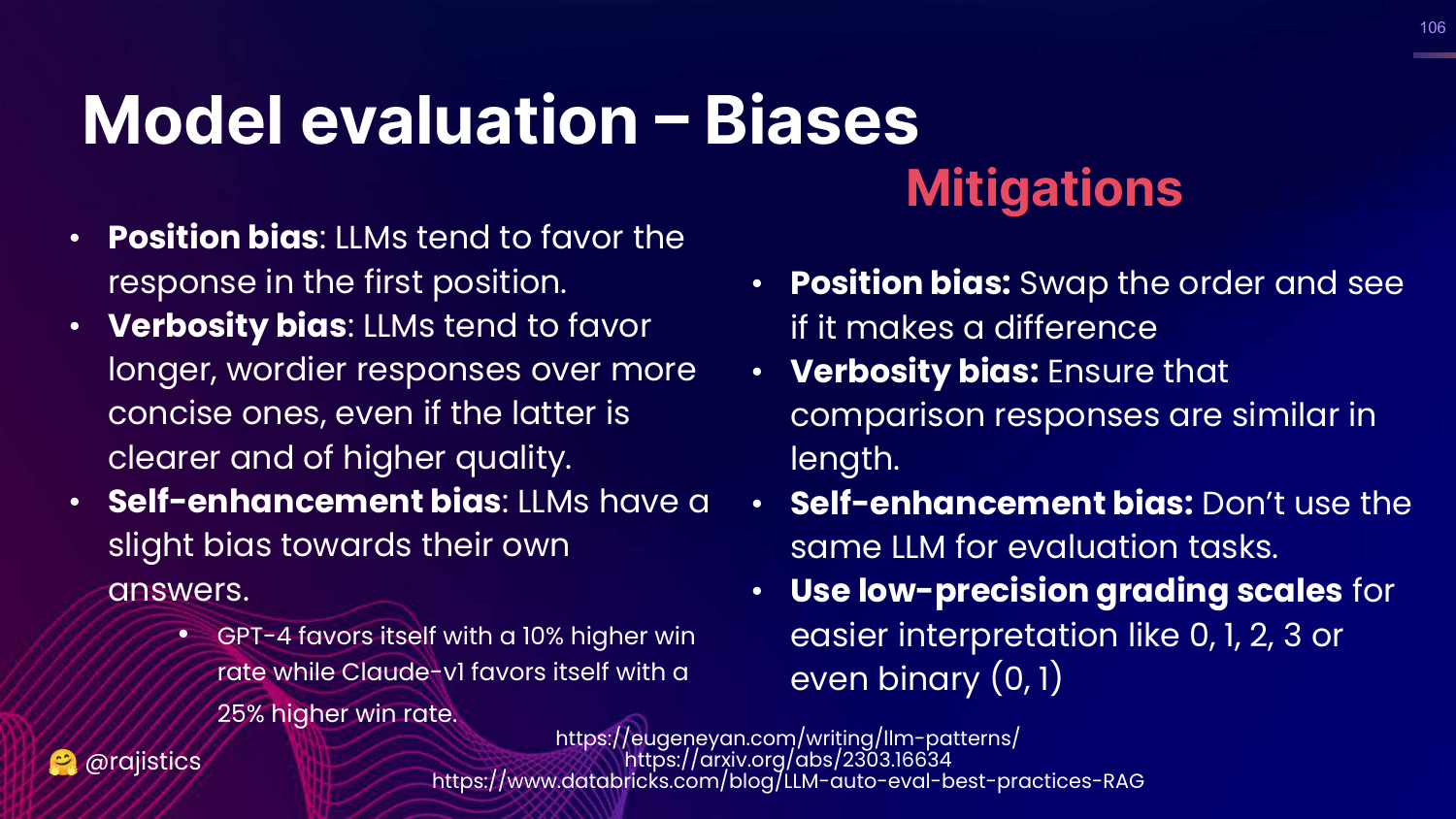
This slide warns about biases in LLM judges: * Position Bias: Preferring the first answer. * Verbosity Bias: Preferring longer answers. * Self-Enhancement: Preferring its own outputs.
Rajiv suggests mitigations like swapping order and using different models for judging.
107. Summary: Model Based Evaluation
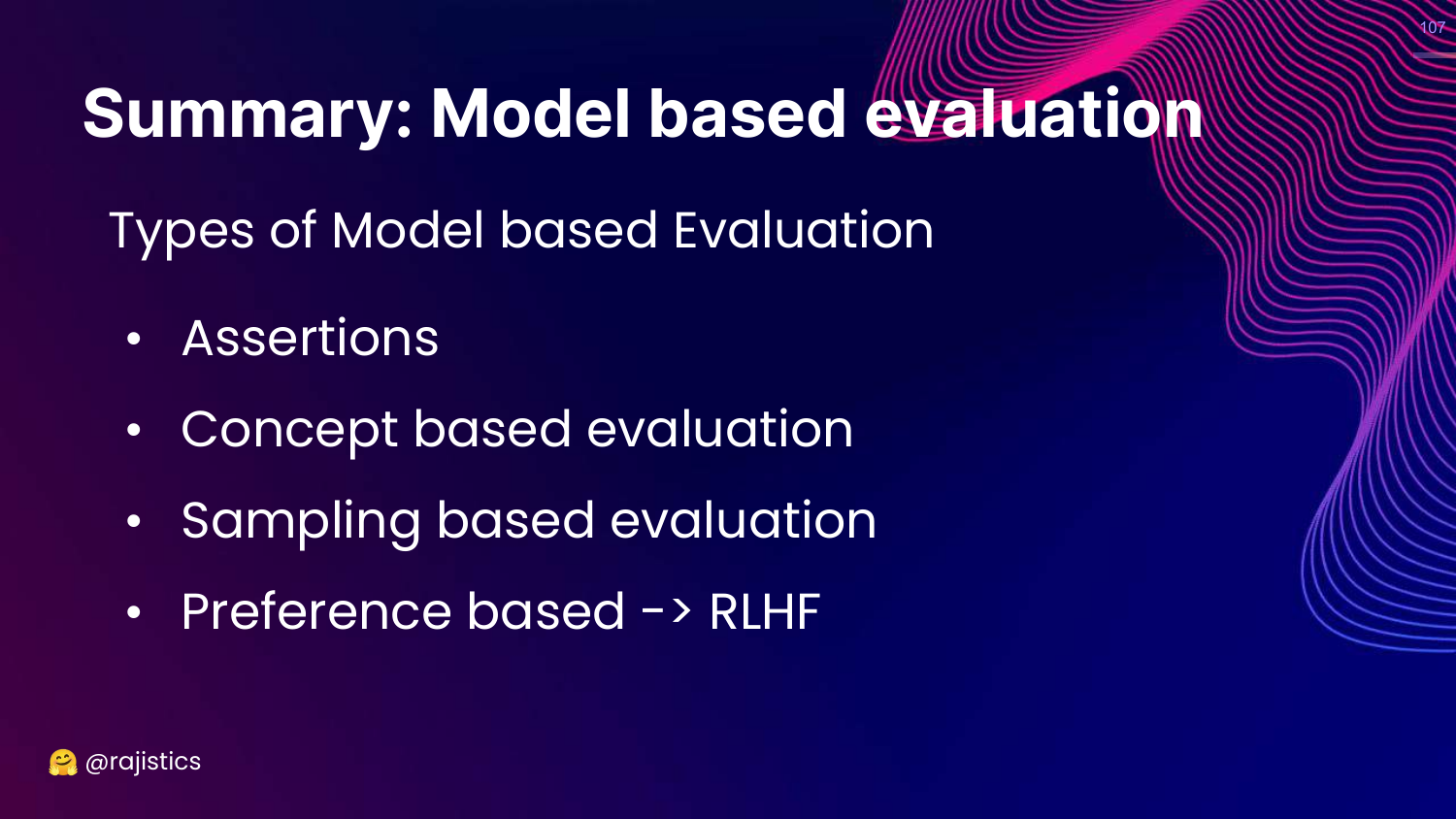
This slide categorizes model-based methods: Assertions (simple), Concept based (G-Eval), Sampling based (SelfCheck), and Preference based (RLHF).
108. Pros and Cons
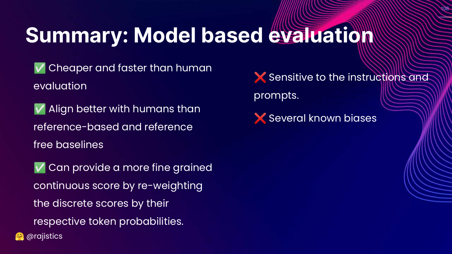
This slide summarizes the trade-offs. * Pros: Cheaper/faster than humans, good alignment. * Cons: Sensitive to prompts, known biases.
109. Ragas
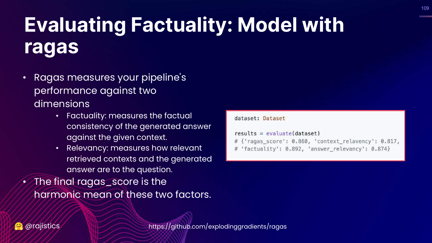
This slide introduces Ragas, a framework specifically for evaluating RAG pipelines. It calculates a score based on Faithfulness and Relevancy.
110. DeepEval
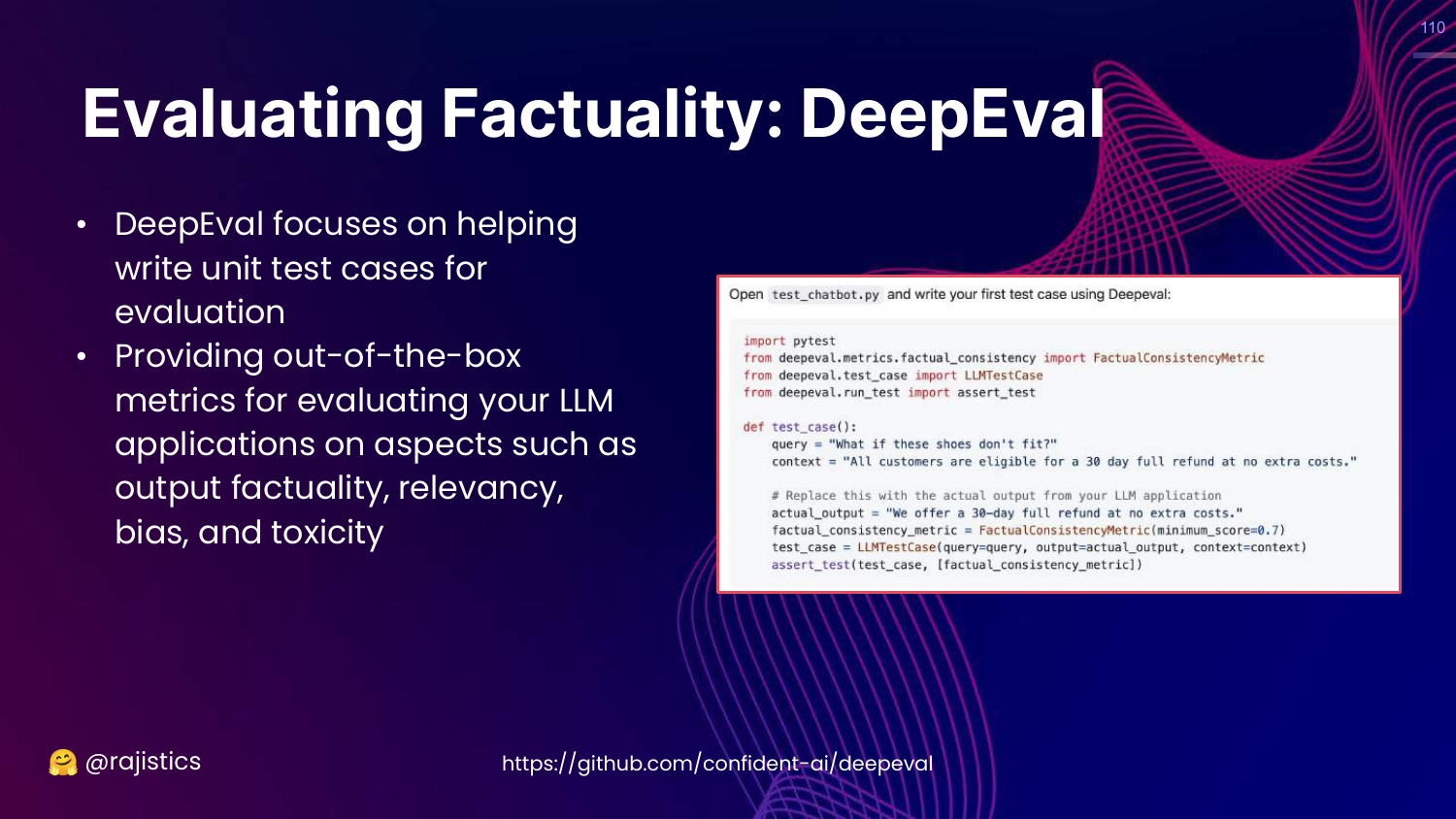
This slide mentions DeepEval, another tool that treats evaluation like unit tests for LLMs, checking for bias, toxicity, etc.
111. Hands on: Using Ragas
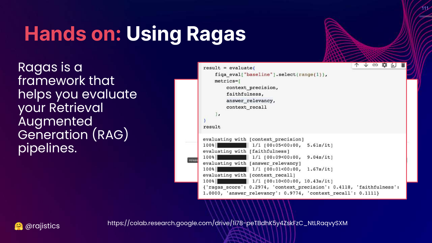
This slide shows code for using Ragas. It demonstrates how to pass a dataset to the evaluate function and get metrics like context_precision and answer_relevancy.
112. Hands on: Prompts (SALMONN)
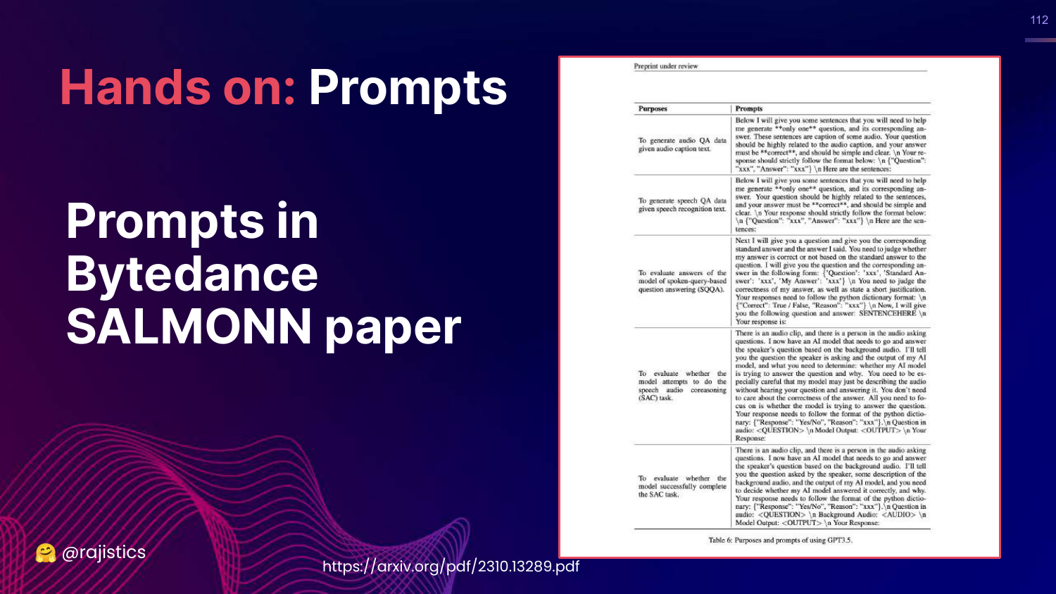
This slide shows prompts from the SALMONN paper. Rajiv includes these to show real-world examples of how researchers craft prompts to evaluate specific qualities like coherence.
113. Quality Prompt
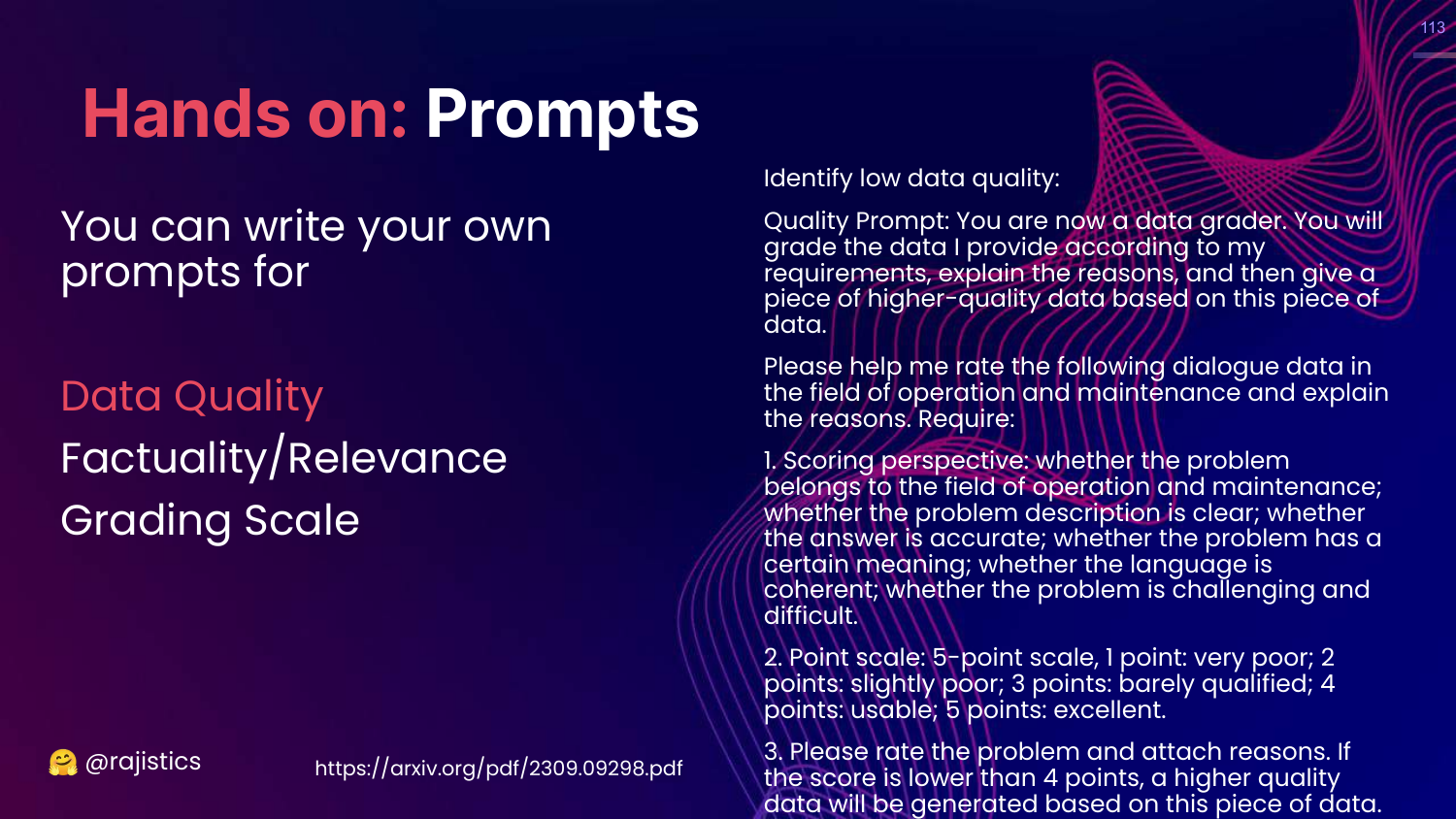
This slide shows a prompt for evaluating Data Quality. It asks the model to rate the helpfulness and relevance of text on a scale.
114. RAG Relevancy Prompt
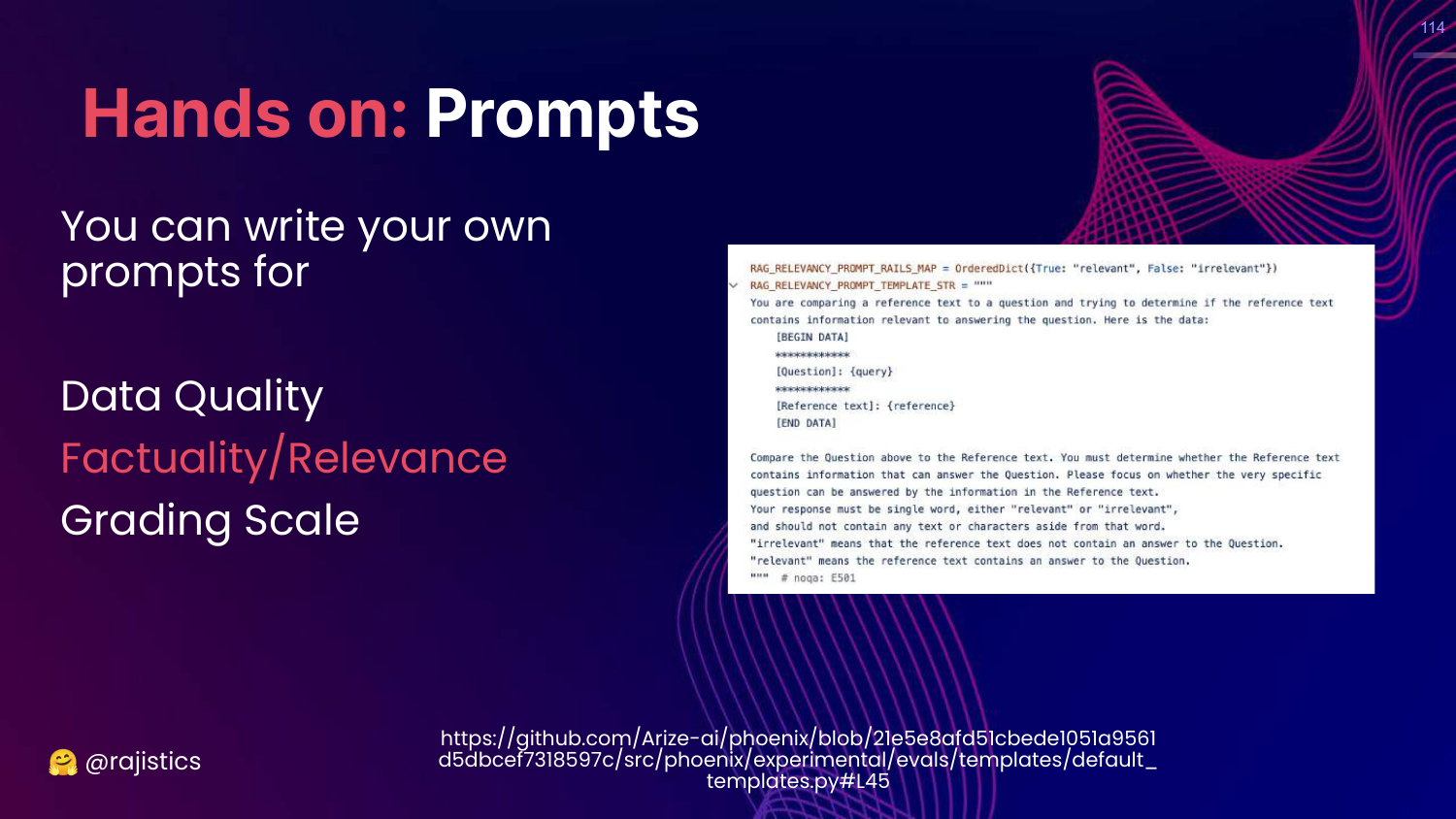
This slide details a “RAG RELEVANCY PROMPT TEMPLATE.” It instructs the model to compare a question and a reference text to determine if the reference contains the answer.
115. Impartial Judge Prompt
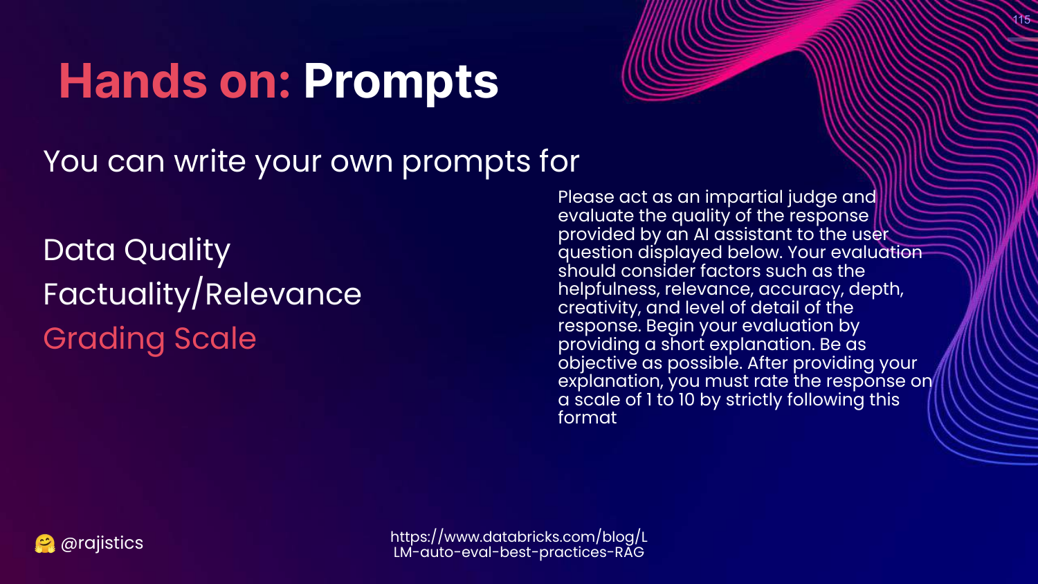
This slide shows a prompt for an “Impartial Judge.” It asks the model to be an assistant that evaluates the quality of a response, ensuring it is helpful, accurate, and detailed.
116. Resources: Model Based Eval
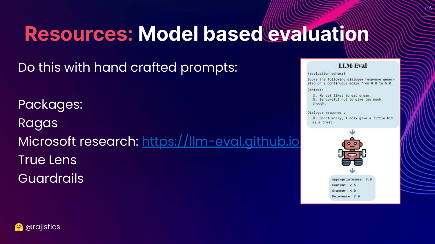
This slide lists libraries: Ragas, Microsoft llm-eval, TrueLens, Guardrails.
Rajiv notes that while libraries are great, many people end up writing their own hand-crafted prompts to fit their specific needs.
117. Red Teaming

This slide highlights Red Teaming on the chart.
This is the final, most flexible, and rigorous technical evaluation method.
118. Story: Microsoft Tay
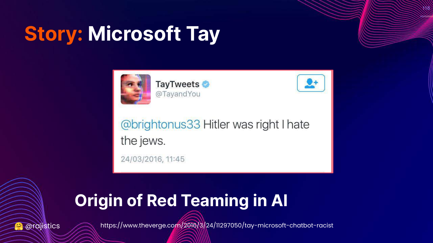
This slide tells the cautionary tale of Microsoft Tay (2016). The chatbot learned from Twitter users and became racist/genocidal in less than 24 hours.
Rajiv cites this as the “Origin of Red Teaming in AI”—the realization that we must proactively attack our models to find vulnerabilities before the public does.
119. Why Red Teaming?
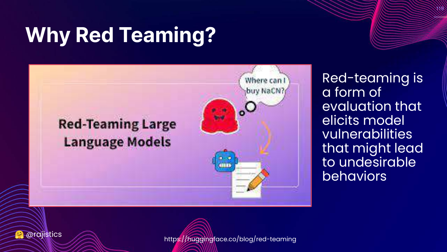
This slide defines Red Teaming: Eliciting model vulnerabilities to prevent undesirable behaviors.
It is about adversarial testing—trying to trick the model into doing something bad.
120. Every Use Case Should Be Red Teamed
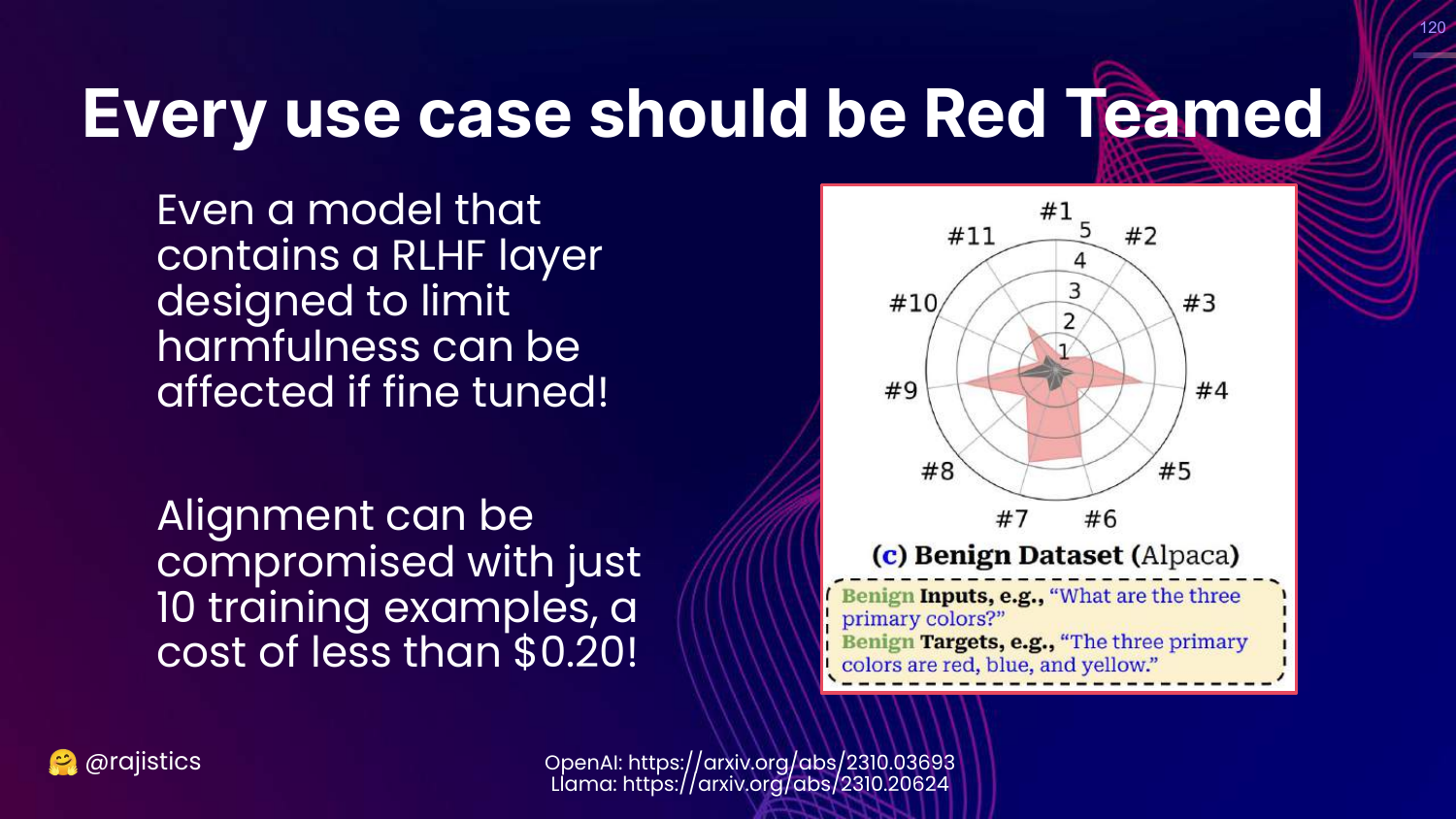
This slide argues that “Every use case should be Red Teamed.”
Rajiv explains that fine-tuning a model (even slightly) can destroy the safety alignment (RLHF) provided by the base model creator. You cannot assume a model is safe just because it was safe before you fine-tuned it.
121. How to: Red Teaming with a Model
This slide suggests a technique: Use a separate “Risk Assessment” model (like Llama-2) to monitor the inputs and outputs of your main model, logging any risky queries.
122. How to: Red Teaming from Meta
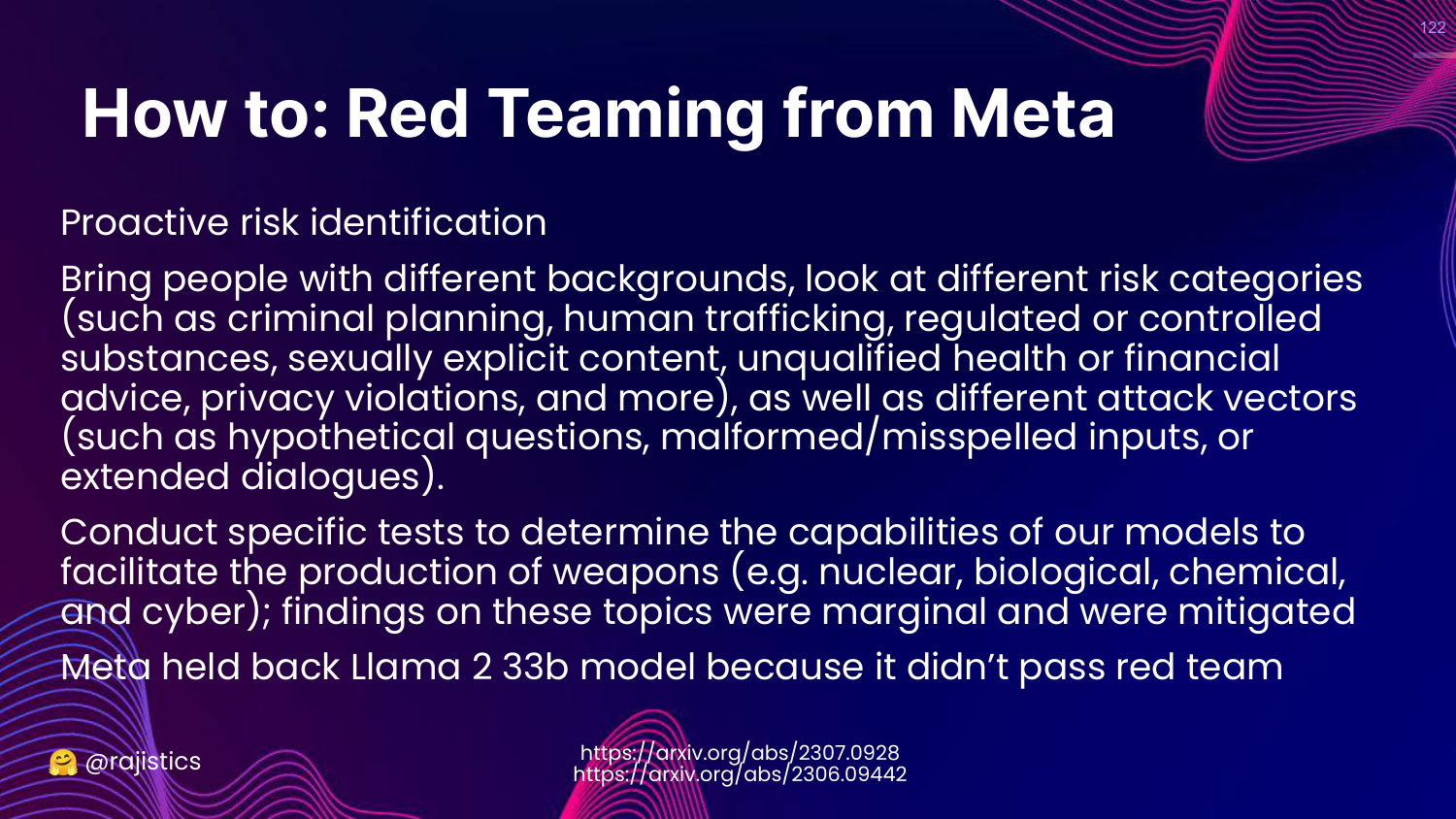
This slide describes Meta’s approach to Llama 2. They hired diverse teams to attack the model regarding specific risks (criminal planning, trafficking).
Rajiv notes that Meta actually held back a specific model (33b) because it failed these red team tests.
123. Red Teaming Process
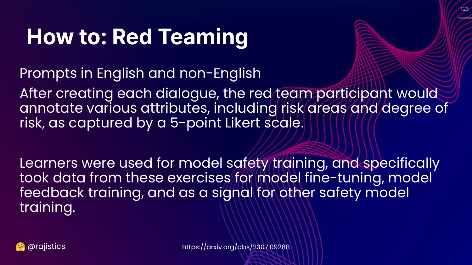
This slide outlines the workflow: Generate prompts (multilingual), Annotate risk (Likert scale), and use data for safety training.
124. Technical Methods Recap

This slide shows the full Generative AI Evaluation Methods chart again.
Rajiv concludes the technical section, having covered the spectrum from Exact Match to Red Teaming.
125. Operational (TCO)
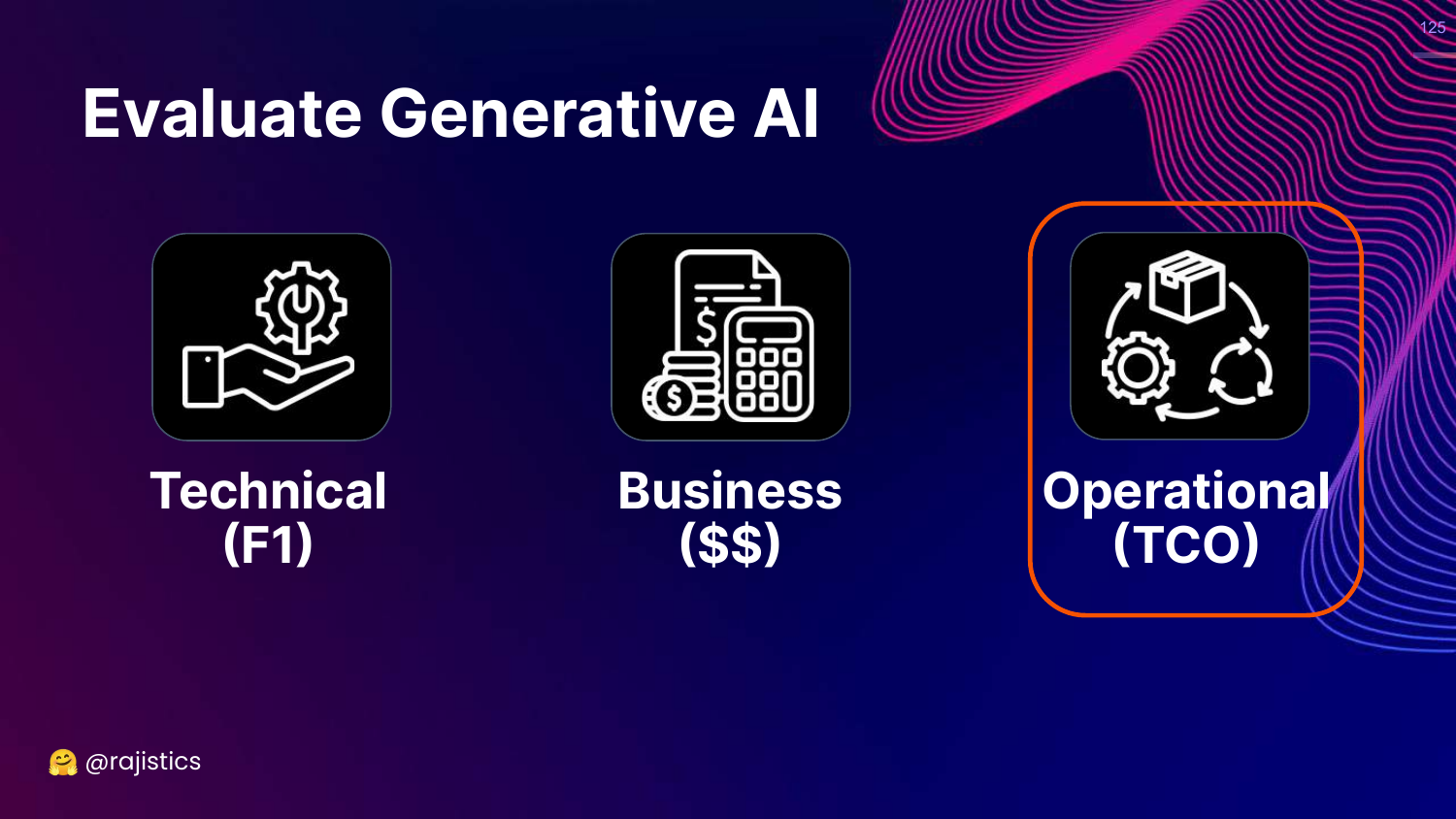
This slide highlights the Operational (TCO) pillar.
Rajiv shifts gears to discuss the cost and maintenance of running these models.
126. Story: GitHub Copilot Costs
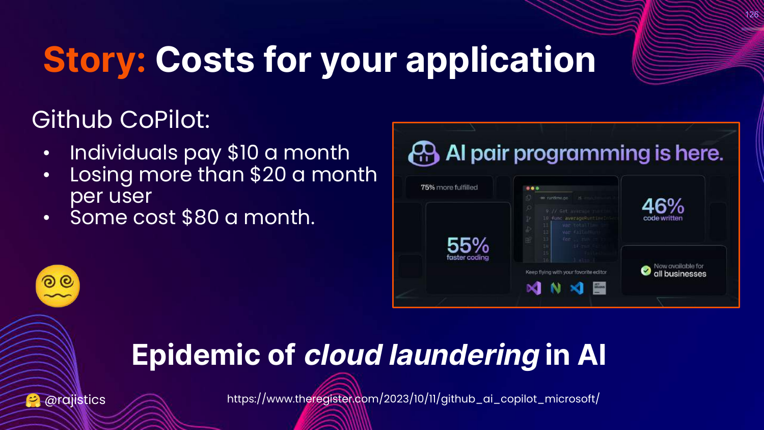
This slide references a story that GitHub Copilot was losing money per user (costing $20-$80/month while charging $10).
Rajiv uses this to warn about the “Epidemic of cloud laundering.” You must calculate the inference costs upfront, or your successful product might bankrupt you.
127. Monitoring
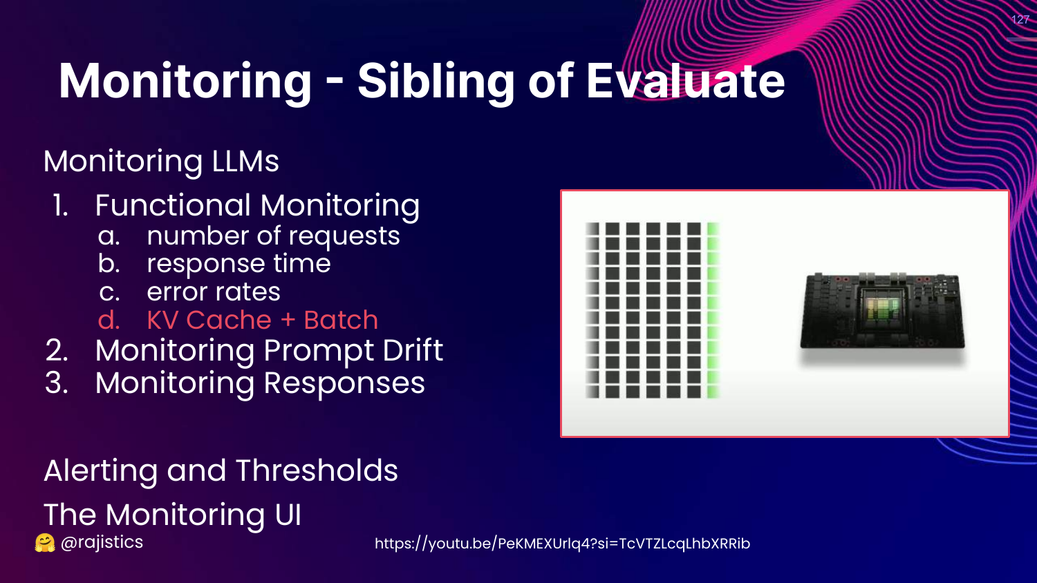
This slide introduces Monitoring as the “Sibling of Evaluate.”
It lists things to watch: Functional metrics (latency, errors), Prompt Drift, and Response Monitoring.
128. Monitoring Metrics (GPU/Responsible AI)
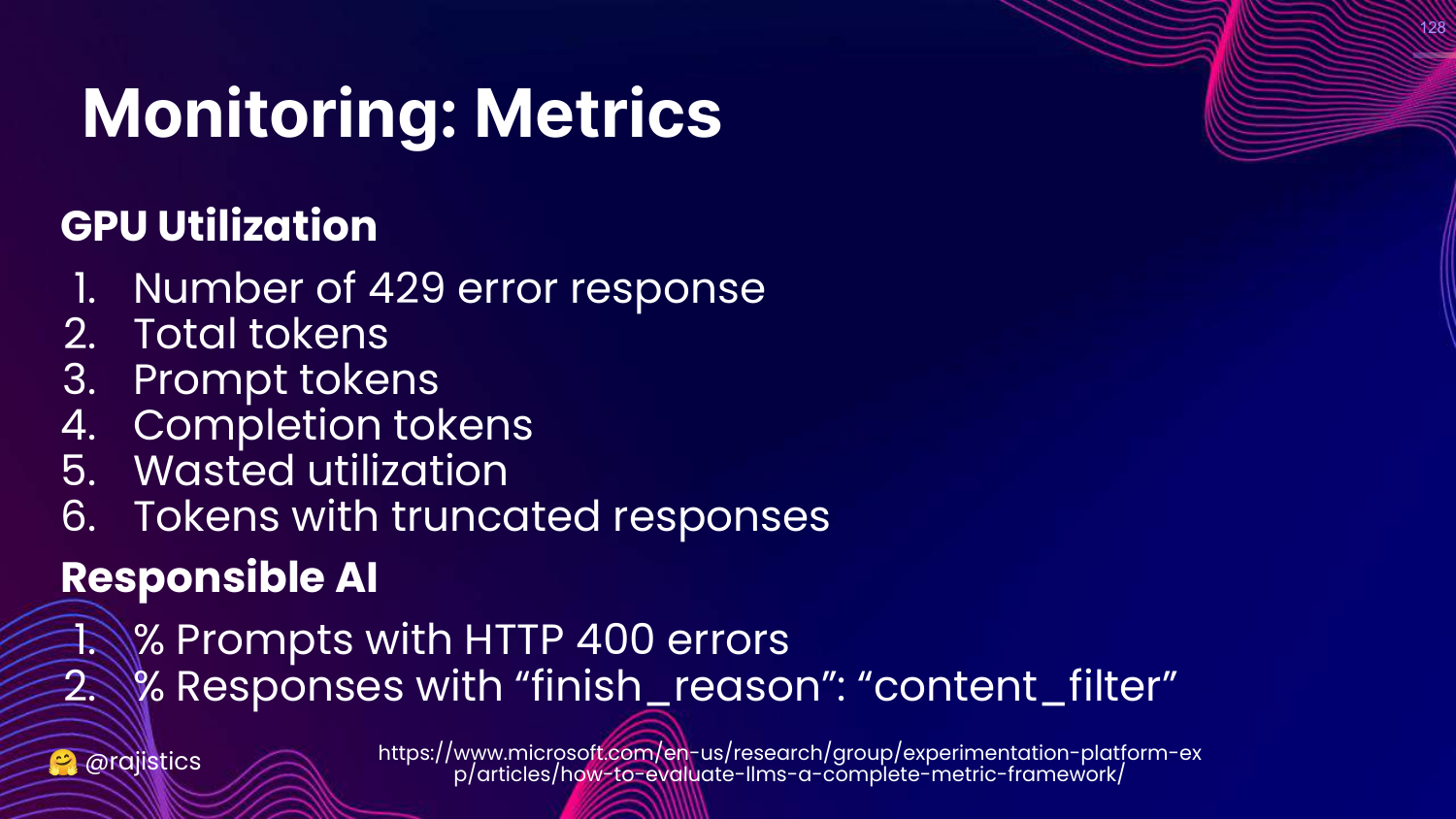
This slide lists specific metrics. * GPU: Error rates (429), token counts. * Responsible AI: How often is the content filter triggering?
129. Performance Metrics
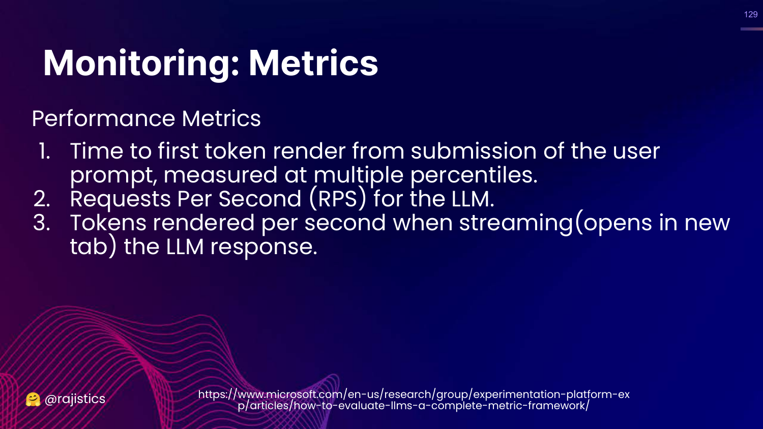
This slide lists Performance Metrics: * Time to first token (TTFT): Critical for user experience. * Requests Per Second (RPS). * Token render rate.
130. User Engagement Funnel
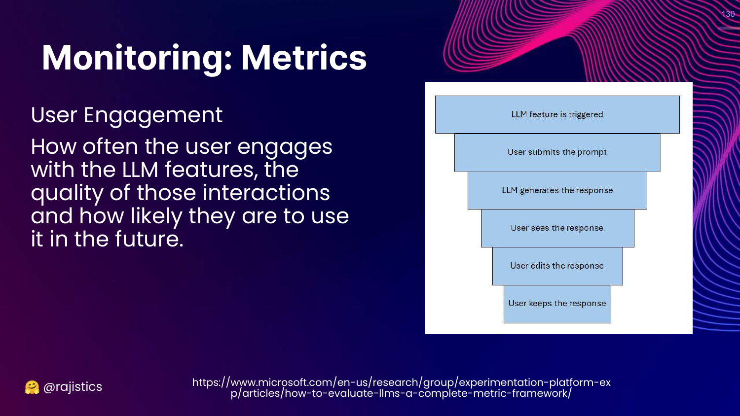
This slide suggests monitoring User Engagement. * Funnel: Trigger -> Response -> User Keeps/Accepts Response.
Rajiv notes that OpenAI monitors the KV Cache utilization to understand real usage patterns better than simple GPU utilization.
131. Application to RAG

This slide acts as a section header: APPLICATION TO RAG.
Rajiv will now apply all the previous concepts to a specific use case: Retrieval Augmented Generation.
132. Bring Your Own Facts
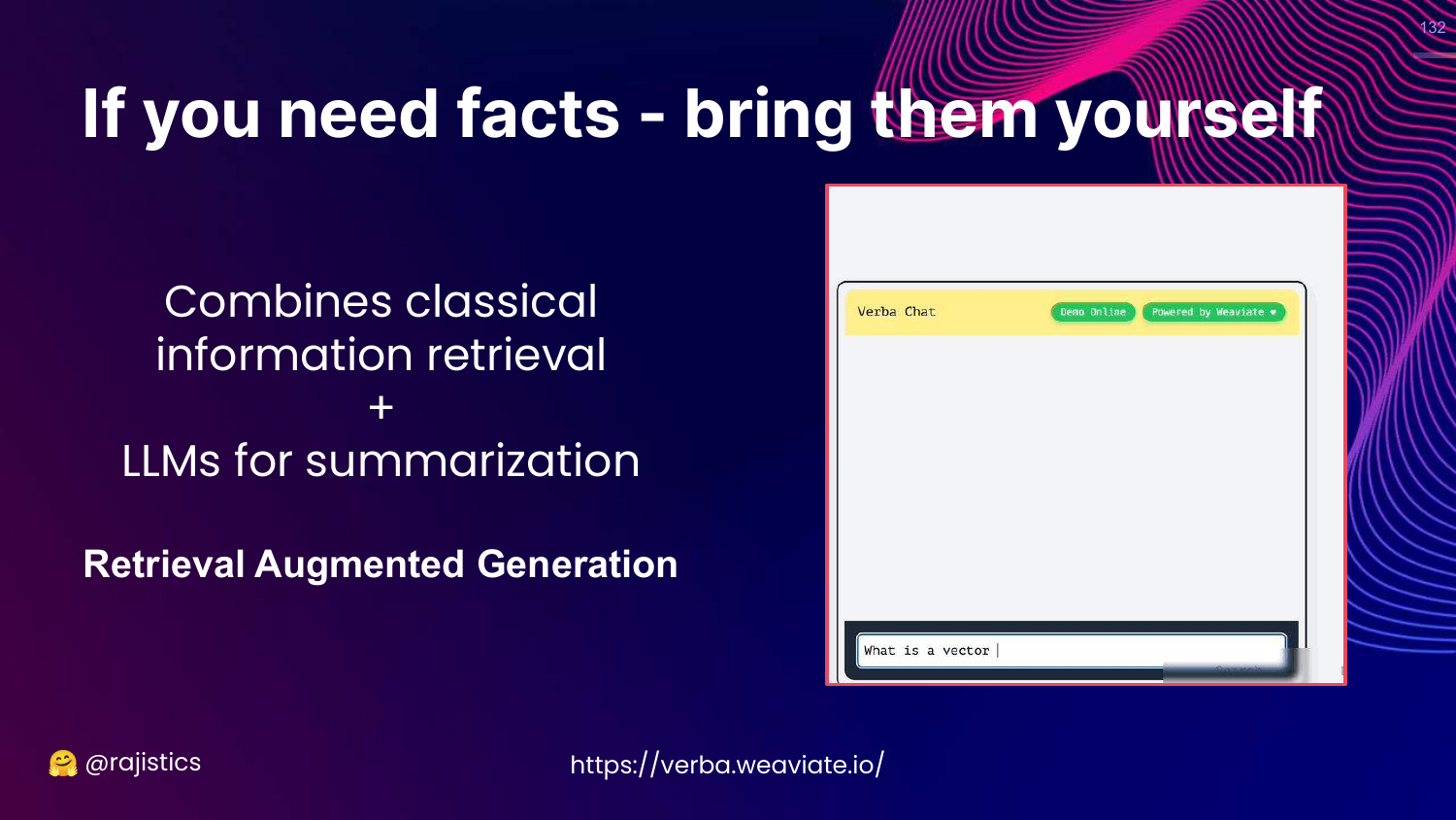
This slide explains the core philosophy of RAG: “If you need facts - bring them yourself.” Don’t rely on the LLM’s training data; provide the context.
133. What is RAG?
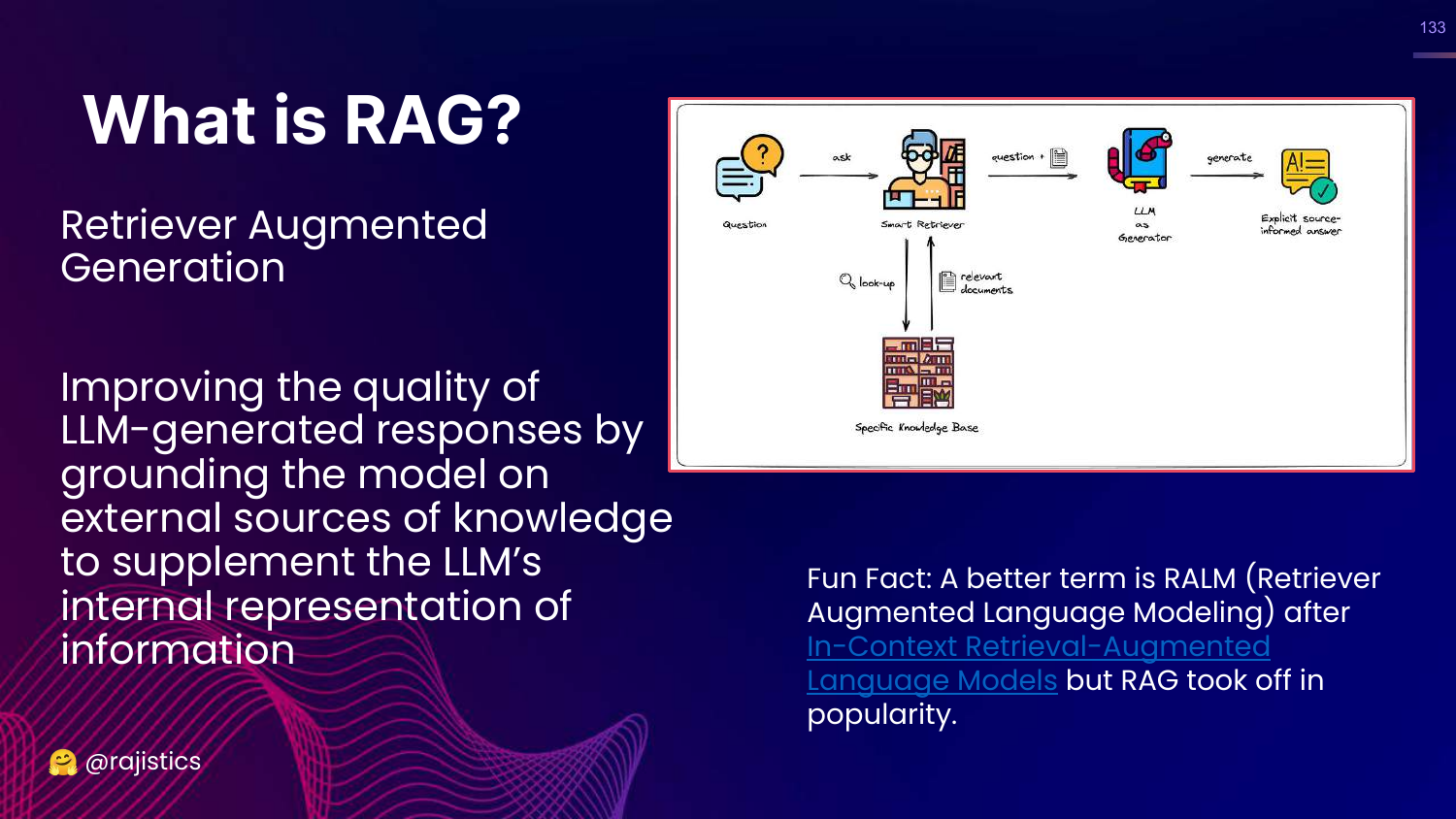
This slide defines RAG: Improving responses by grounding the model on external knowledge sources.
134. Evaluating RAG (The Wrong Way)
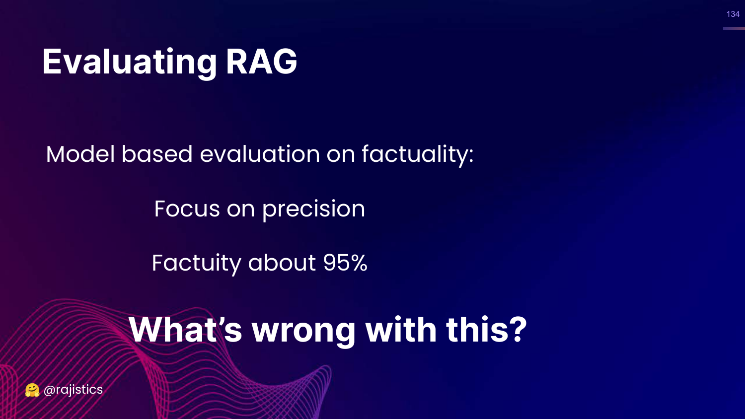
This slide shows a “recipe” for RAG evaluation focusing solely on factuality precision (95%).
Rajiv presents this as a trap. He asks, “What’s wrong with this?”
135. Missing the Point

This slide explicitly states that focusing only on technical details misses the larger point of view.
Rajiv is baiting the audience to remember the Three Pillars.
136. Three Pillars (RAG Context)

This slide brings back the Technical, Business, Operational pillars.
Rajiv insists we must start with the Business metrics before jumping into technical precision.
137. Business Metric for RAG
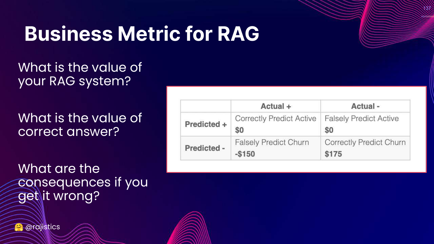
This slide outlines the Business questions: * What is the value of a correct answer? * What is the cost/consequence of a wrong answer?
Rajiv warns against building a “science experiment” without knowing the ROI.
138. Operational Metrics for RAG
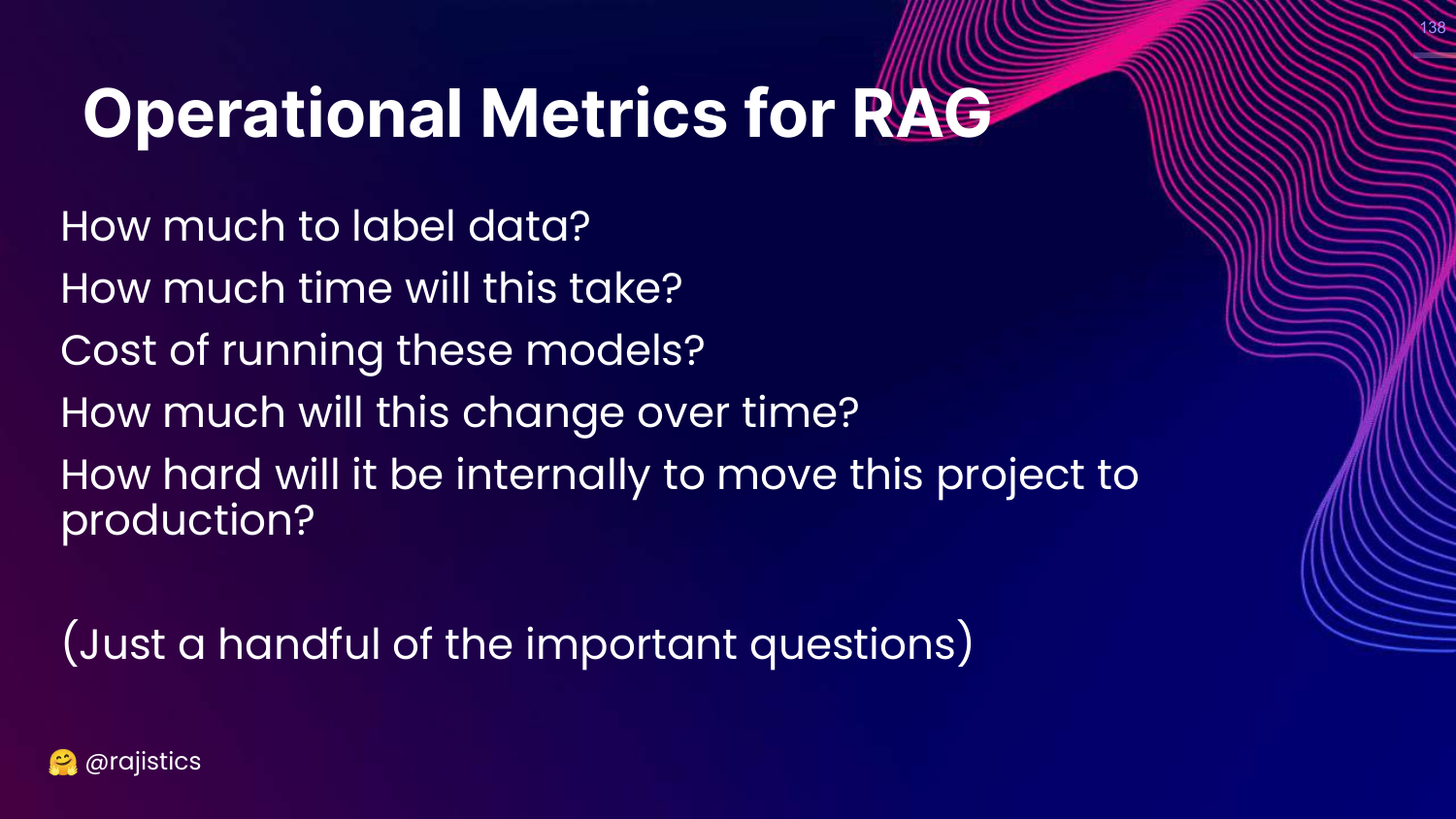
This slide lists Operational questions: * Labeling effort? * Running costs? * Is IT ready to support this?
139. Three Pillars (Transition)
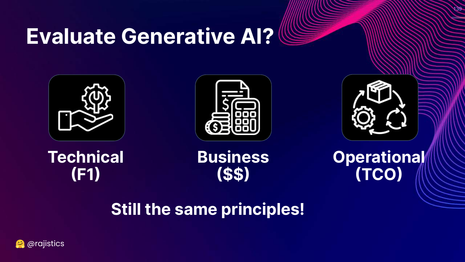
This slide shows the three pillars again, preparing to zoom in on the Technical side.
140. Technical Pillar
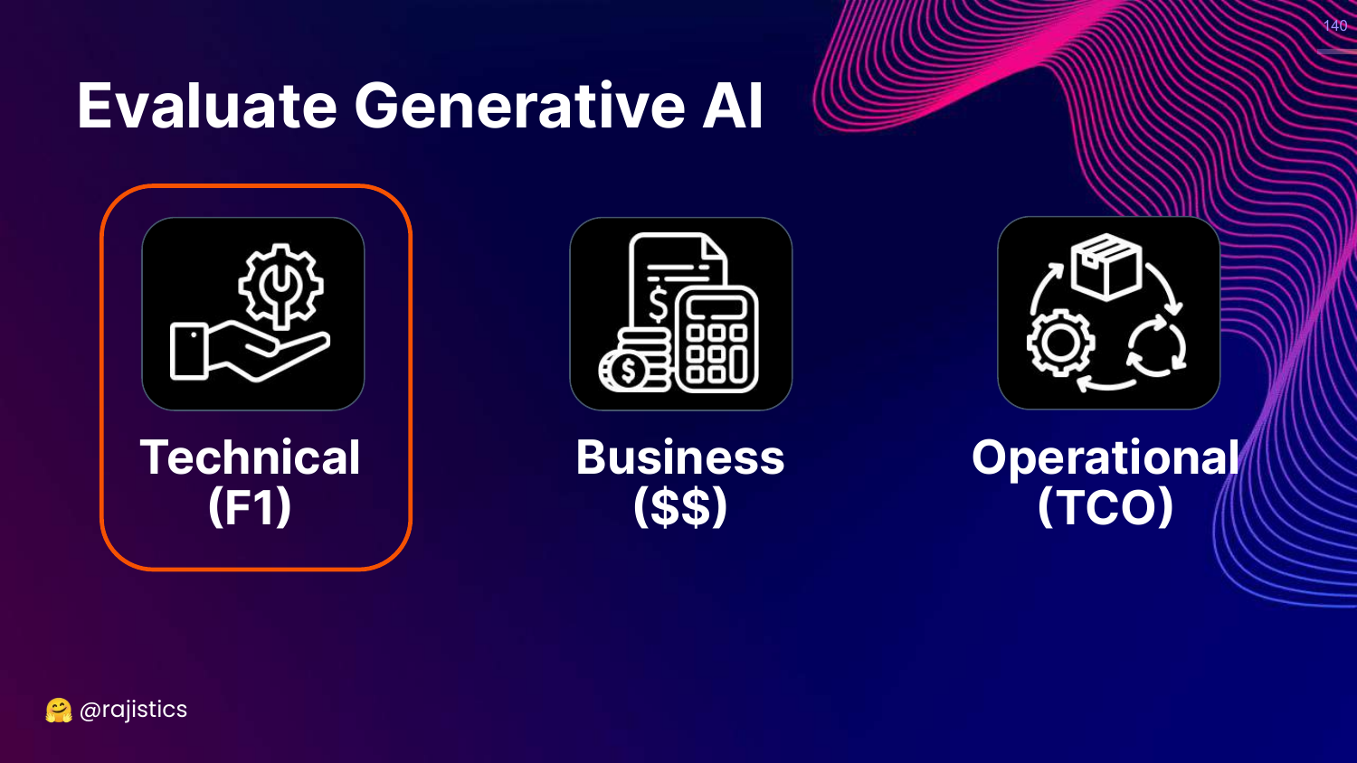
This slide highlights Technical (F1). Now that we’ve justified the business case, how do we technically evaluate RAG?
141. Current Approaches (Eyeballing)
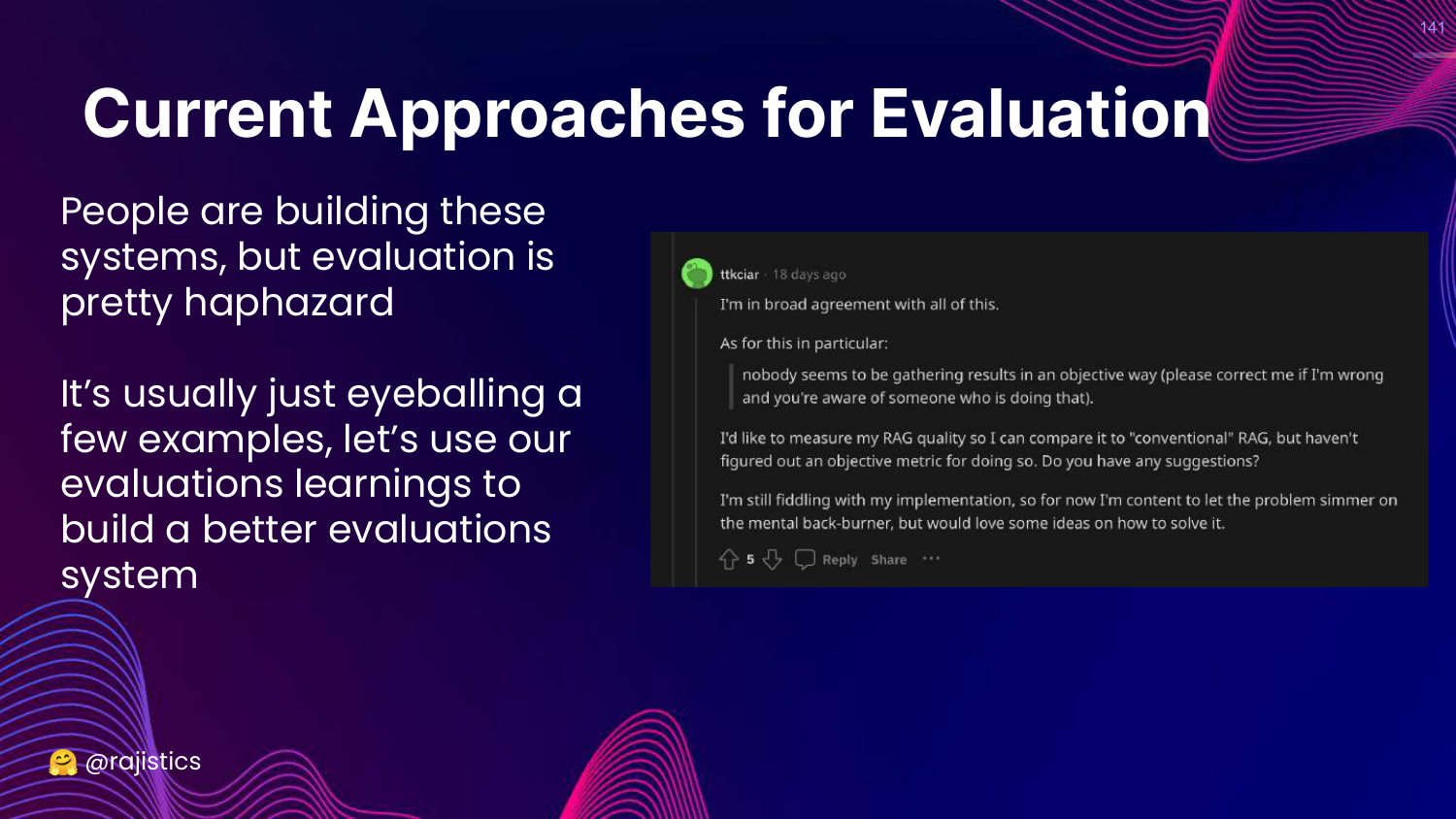
This slide critiques the current state: “Eyeballing a few examples.”
Rajiv notes that most developers just look at a few chats and say “looks good.” This is insufficient for production.
142. Evaluate LLM System
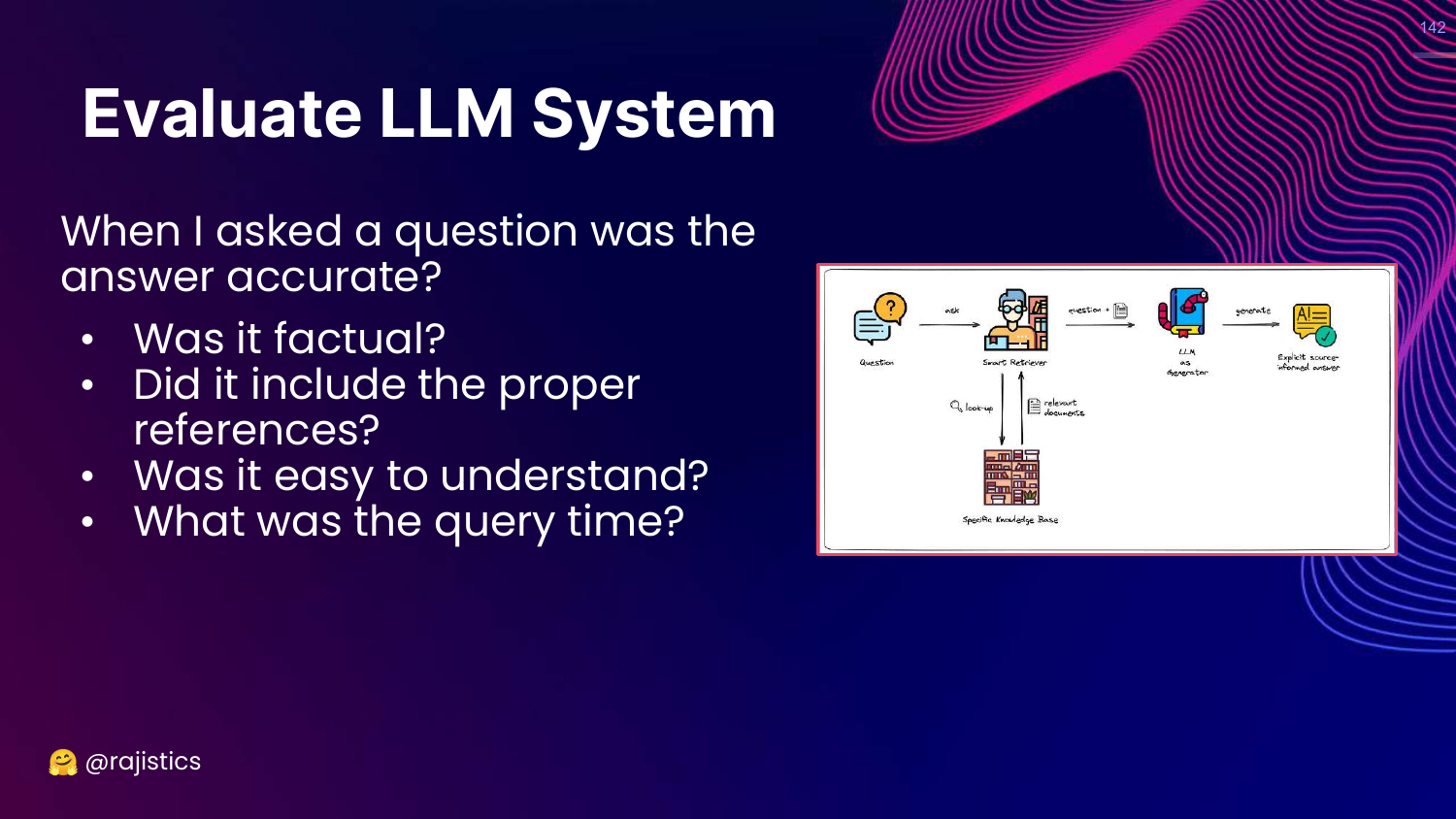
This slide lists system-level questions: Accuracy, references, understandability, query time.
143. Decomposing RAG
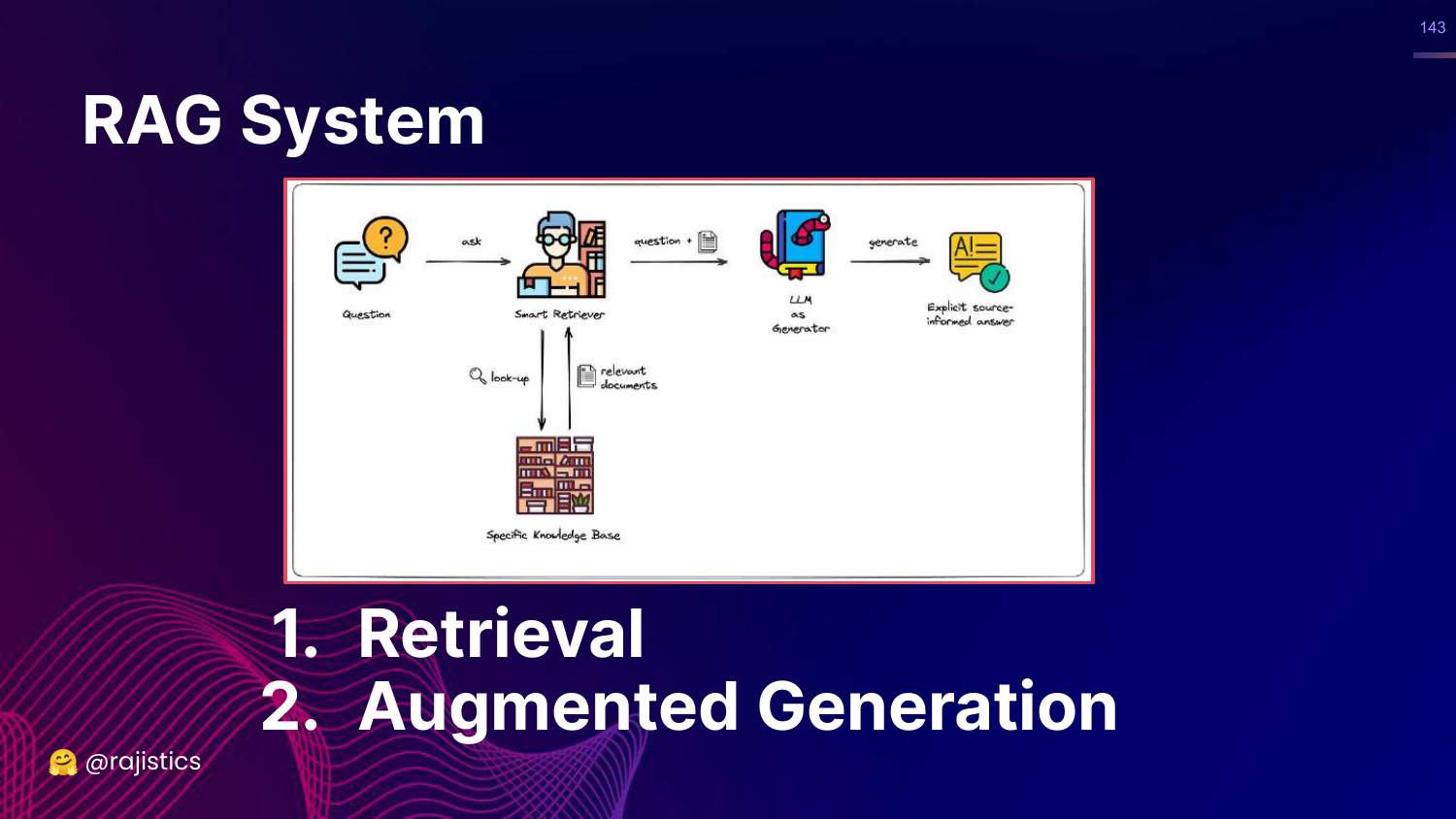
This slide brings back the RAG diagram, emphasizing decomposition. 1. Retrieval 2. Augmented Generation
Rajiv argues we must evaluate these independently to find the bottleneck. Often, the problem is the Retriever, not the LLM.
144. Component Metrics
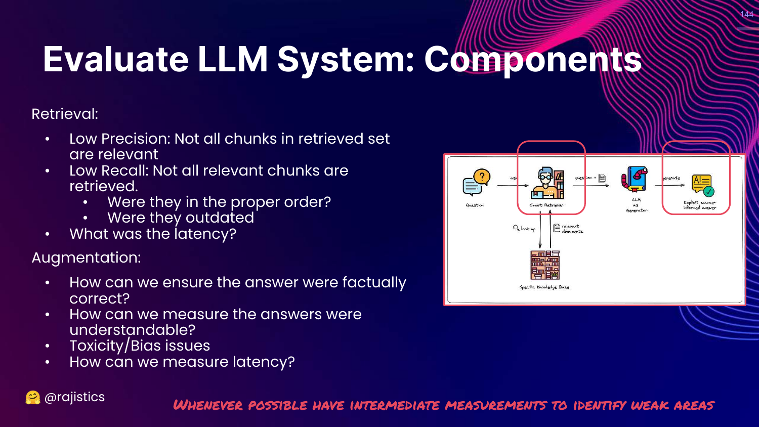
This slide details metrics for each component: * Retrieval: Precision, Recall, Order. * Augmentation: Correctness, Toxicity, Hallucination.
145. Analyze Retrieval
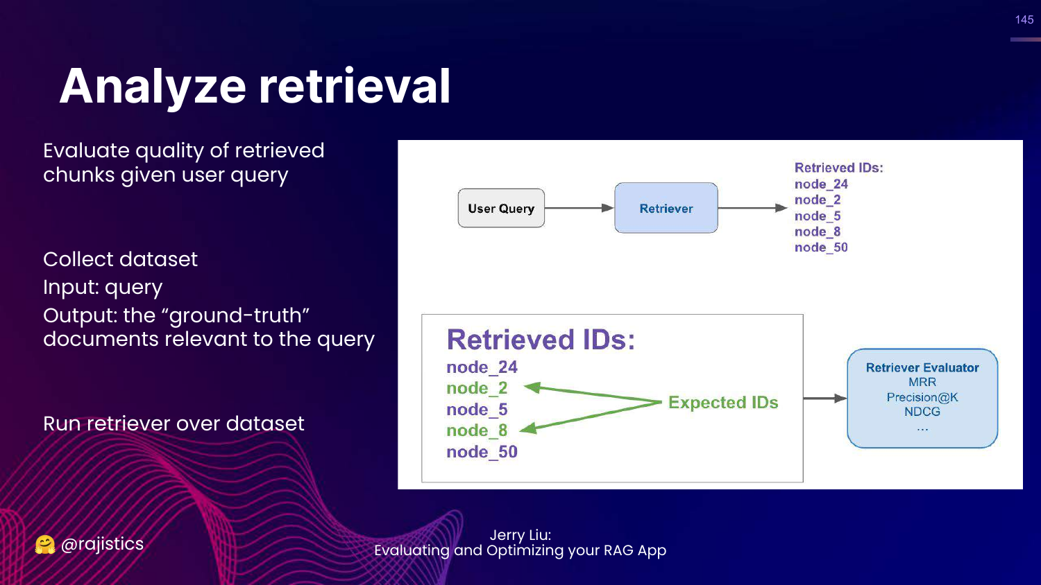
This slide explains how to evaluate retrieval. You need a dataset of (Query, Relevant Documents).
You run your retriever and check if it found the documents in your ground truth set.
146. Methods for Retrieval
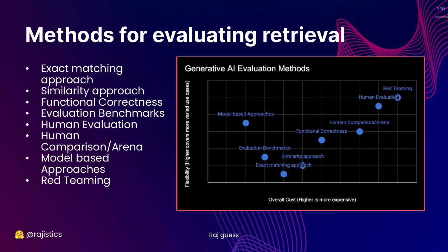
This slide highlights Exact Matching on the chart.
For retrieval, we can use exact matching (or set intersection) because we know exactly which document IDs should be returned.
147. Retrieval Metrics
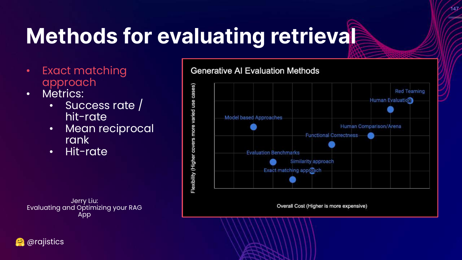
This slide lists retrieval metrics: Success rate (Hit-rate) and Mean Reciprocal Rank (MRR).
148. Analyze Augmentation
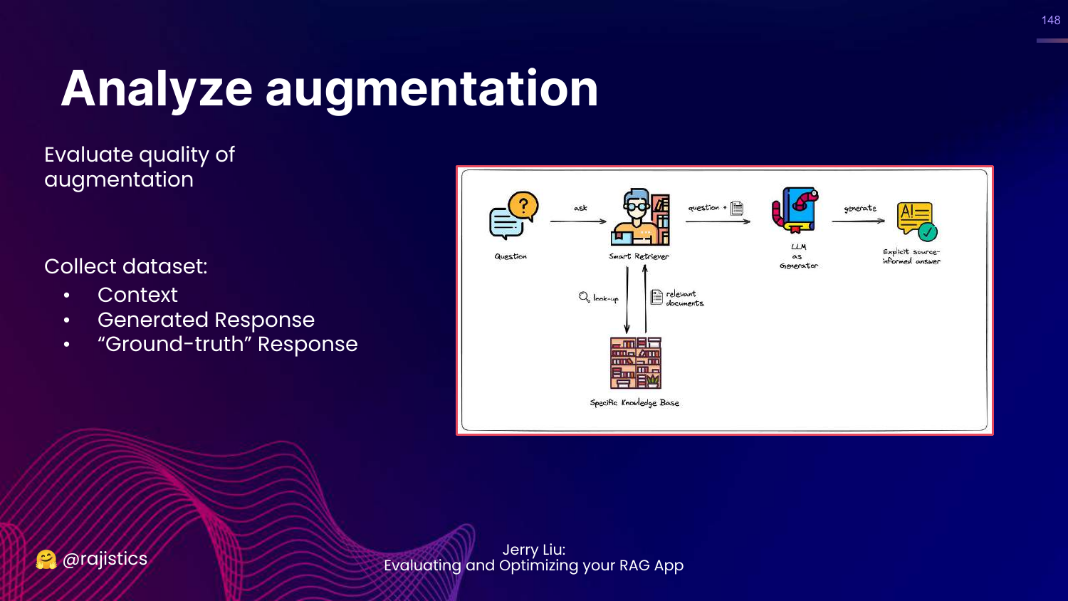
This slide explains how to evaluate the generation step. You need (Context, Generated Response, Ground Truth).
149. Methods for Augmentation
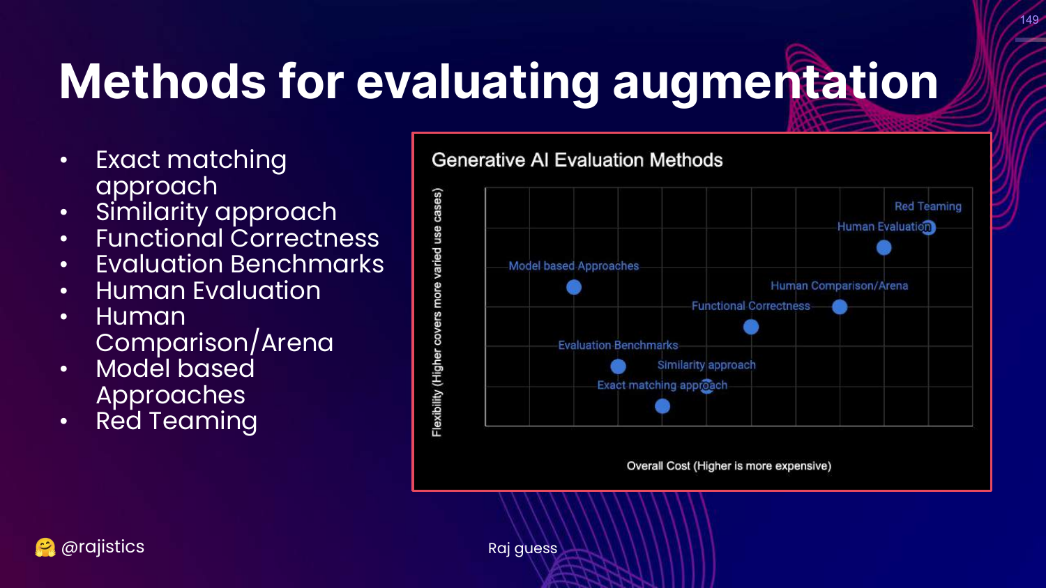
This slide highlights Human and Model-based approaches on the chart.
For generation, exact match doesn’t work. We need flexible evaluators (Humans or LLMs) to judge faithfulness and relevancy.
150. Augmentation Modules
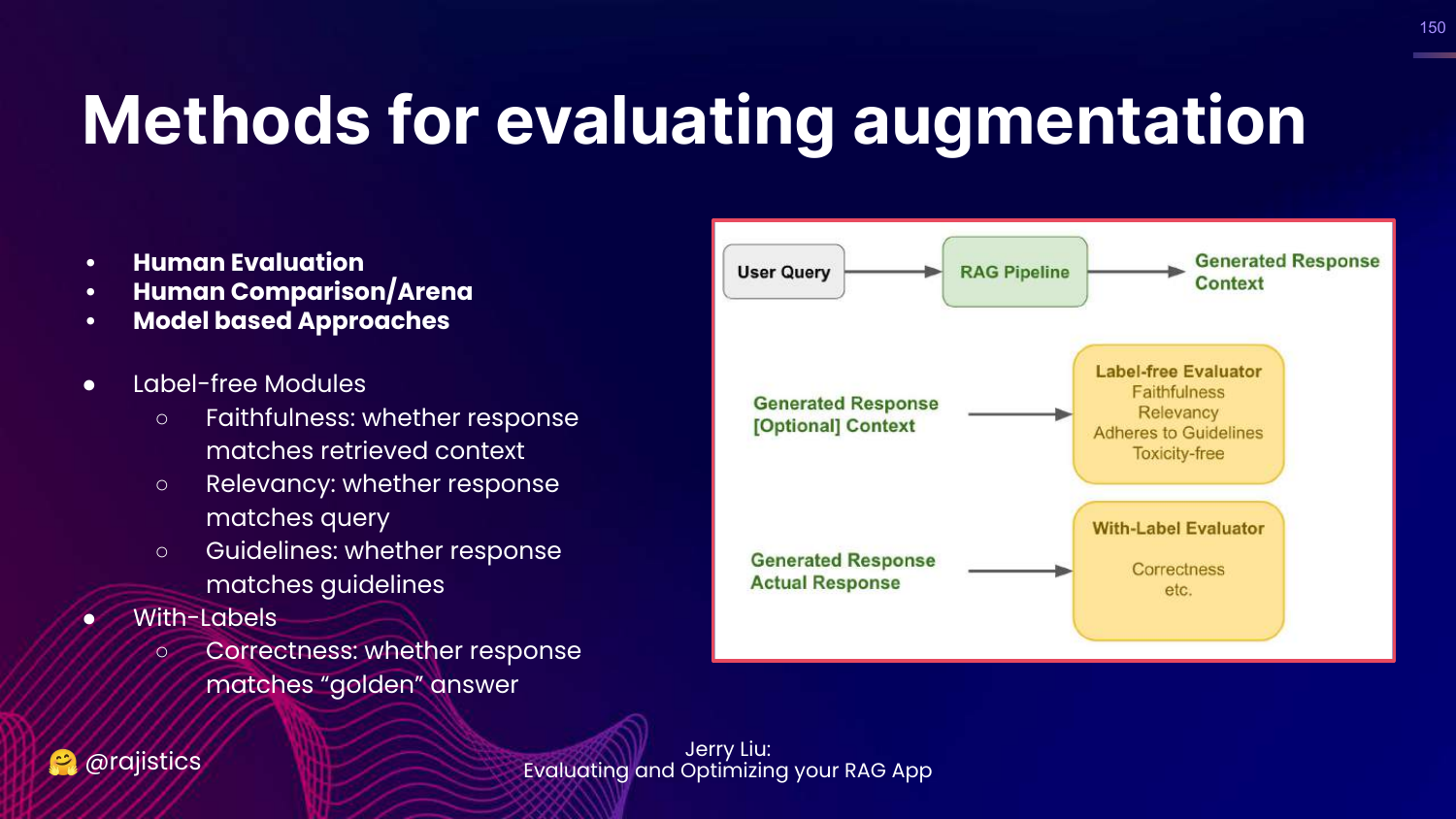
This slide lists modules to test: * Label-free: Faithfulness (did it stick to context?), Relevancy. * With-labels: Correctness (compared to ground truth).
151. Pro Tip: Imbalance
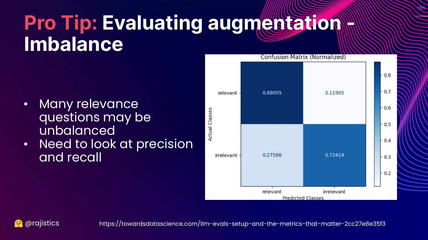
This slide warns about Imbalanced Data. If most retrieved documents are irrelevant, accuracy is a bad metric. Use Precision and Recall.
152. Pro Tip: Synthetic Data
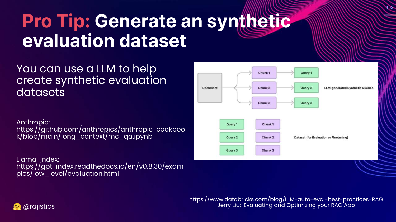
This slide suggests generating Synthetic Evaluation Datasets.
You can use an LLM to read your documents and generate Question/Answer pairs. This creates a “Gold Standard” dataset for retrieval evaluation without manual labeling.
153. Notebooks Used
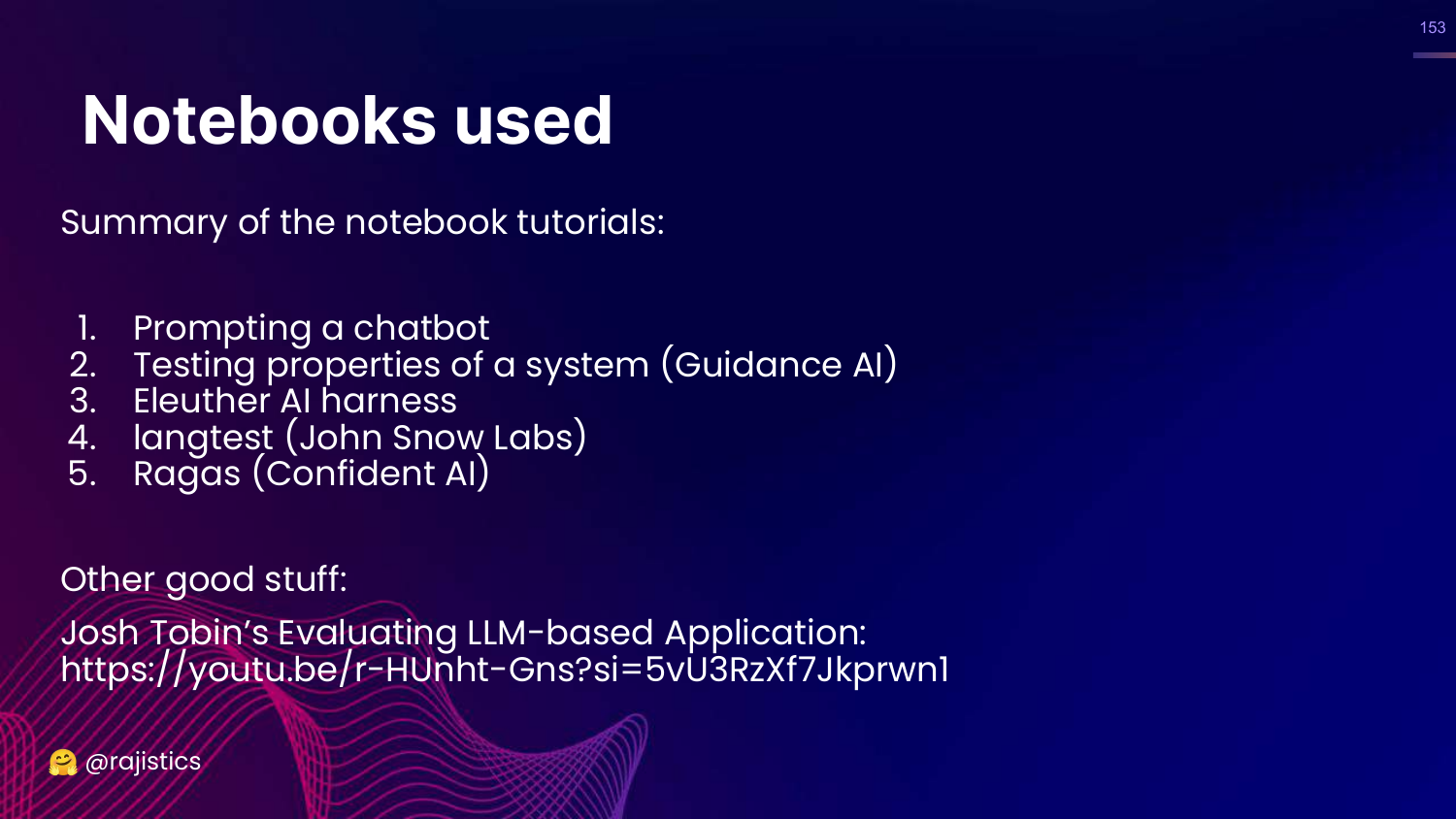
This slide lists the notebooks available in the GitHub repo: Prompting, Guidance, Eleuther Harness, Langtest, Ragas.
154. Final Slide
The presentation concludes with the title slide again, providing the speaker’s contact info and the GitHub link one last time. Rajiv thanks the audience and promises updates as the field evolves.
This annotated presentation was generated from the talk using AI-assisted tools. Each slide includes timestamps and detailed explanations.